Analyze growth of LCLs
Briana Mittleman
2018-03-16
Last updated: 2018-03-21
Code version: 93a4722
library(dplyr)
Attaching package: 'dplyr'The following objects are masked from 'package:stats':
filter, lagThe following objects are masked from 'package:base':
intersect, setdiff, setequal, unionlibrary(tidyr)
library(ggplot2)
library(reshape2)Warning: package 'reshape2' was built under R version 3.4.3
Attaching package: 'reshape2'The following object is masked from 'package:tidyr':
smithsgrowth=read.csv("../data/growth_curve_3.16.csv", header = TRUE)
#filter out control
growth_e= growth %>% filter(control=="e") %>% mutate(avg_h=(h_18486+ h_18499 + h_18502 + h_18504 + h_18510 + h_18517 + h_18523)/7) %>% mutate(avg_c=(c_c3641 + c_pt30 + c_pt91 + c_3610 + c_3659 + c_3622 + c_18358 + c_18359)/8)plot(growth_e$avg_h, xlab="Day", ylim=c(0,2), ylab="cells/ml 10^6", main="Human growth by day")
lines(growth_e$h_18486, col="red")
lines(growth_e$h_18499, col="orange")
lines(growth_e$h_18502, col="yellow")
lines(growth_e$h_18504, col="green")
lines(growth_e$h_18510, col= "blue")
lines(growth_e$h_18517, col="purple")
lines(growth_e$h_18523, col="pink")
plot(growth_e$avg_c, xlab="Day", ylim=c(0,3), ylab="cells/ml 10^6", main="Chimp Growth by day")
lines(growth_e$c_c3641, col="red")
lines(growth_e$c_pt30, col="orange")
lines(growth_e$c_pt91, col="yellow")
lines(growth_e$c_3610, col="green")
lines(growth_e$c_3659, col= "blue")
lines(growth_e$c_18358, col="purple")
lines(growth_e$c_18359, col="pink")
lines(growth_e$c_3622, col="black")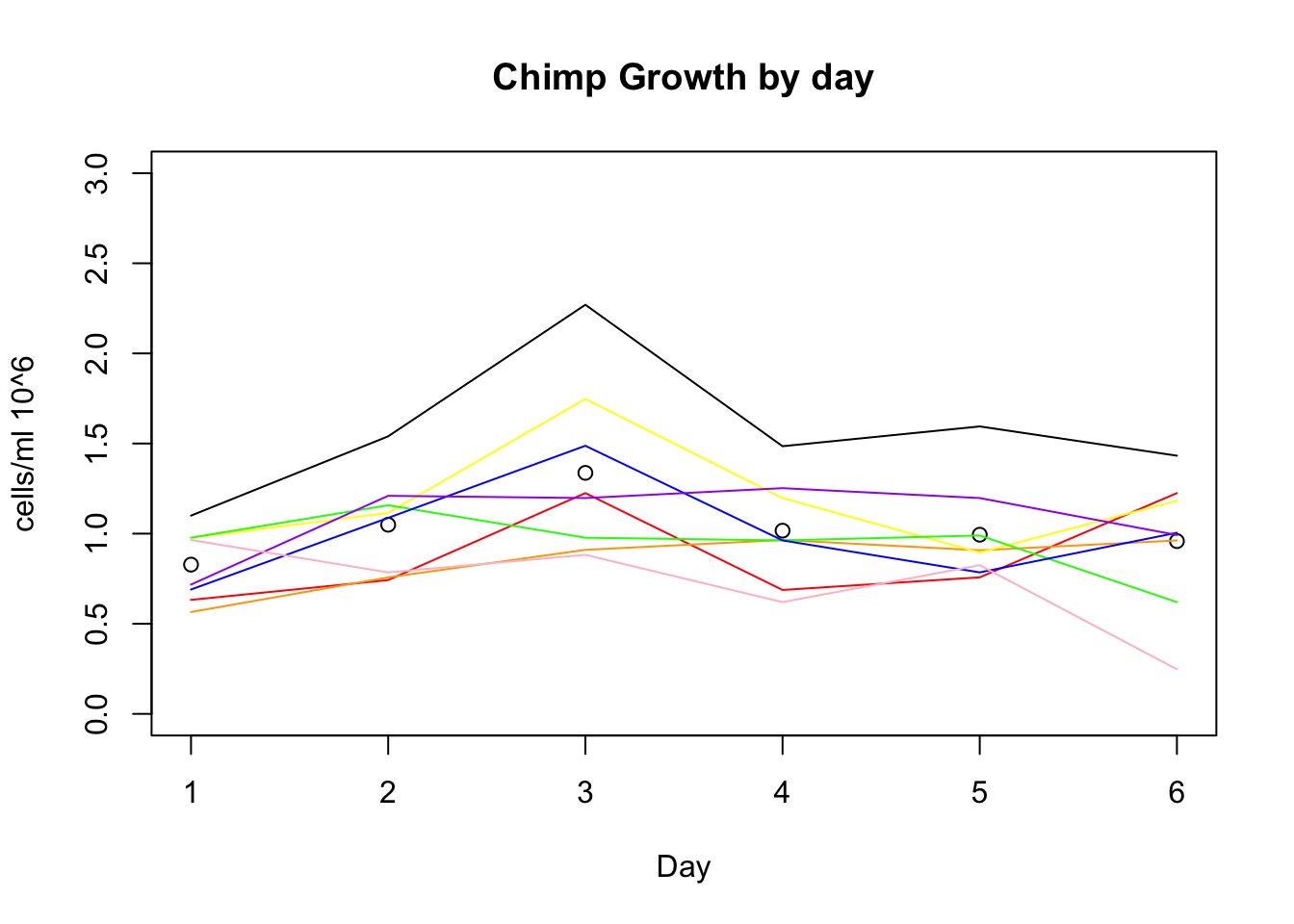
alive=read.csv("../data/perc_alive_3.16.csv", header=TRUE)
alive_e= alive %>% filter(control=="e") %>% mutate(avg_h=(h_18486+ h_18499 + h_18502 + h_18504 + h_18510 + h_18517 + h_18523)/7) %>% mutate(avg_c=(c_c3641 + c_pt30 + c_pt91 + c_3610 + c_3659 + c_3622 + c_18358 + c_18359)/8)plot(alive_e$avg_h, xlab="Day", ylim=c(50,100), ylab="Percent living", main="Human perc living by day")
lines(alive_e$h_18486, col="red")
lines(alive_e$h_18499, col="orange")
lines(alive_e$h_18502, col="yellow")
lines(alive_e$h_18504, col="green")
lines(alive_e$h_18510, col= "blue")
lines(alive_e$h_18517, col="purple")
lines(alive_e$h_18523, col="pink")
abline(v=3,lwd=3, lty=2)
plot(alive_e$avg_c, xlab="Day", ylim=c(0,100), ylab="Percent living", main="Chimp perc living by day")
lines(alive_e$c_c3641, col="red")
lines(alive_e$c_pt30, col="orange")
lines(alive_e$c_pt91, col="yellow")
lines(alive_e$c_3610, col="green")
lines(alive_e$c_3659, col= "blue")
lines(alive_e$c_18358, col="purple")
lines(alive_e$c_18359, col="pink")
lines(alive_e$c_3622, col="black")
abline(v=3,lwd=3, lty=2)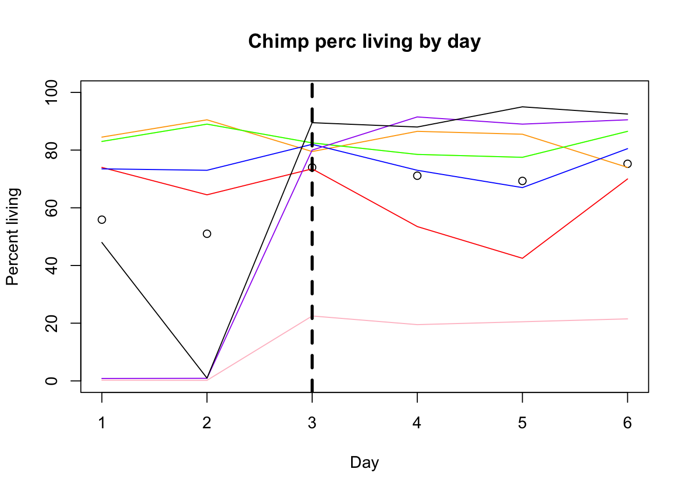
plot(alive_e$avg_h ~ growth_e$avg_h, ylab="Percent living", xlab="Concentration", ylim=c(50,100), pch=16, main="Human Percent living vs Concentration")
points(alive_e$h_18486 ~ growth_e$h_18486, col="red", pch=16)
points(alive_e$h_18499 ~ growth_e$h_18499, col="orange", pch=16)
points(alive_e$h_18502 ~ growth_e$h_18502, col="yellow", pch=16)
points(alive_e$h_18504 ~ growth_e$h_18504, col="green", pch=16)
points(alive_e$h_18510 ~ growth_e$h_18510, col="blue", pch=16)
points(alive_e$h_18517 ~ growth_e$h_18517, col="purple", pch=16)
points(alive_e$h_18523 ~ growth_e$h_18523, col="pink", pch=16)
reg= lm(alive_e$avg_h~ growth_e$avg_h)
coeff=coefficients(reg)
eq = paste0("y = ", round(coeff[2],1), "*x +", round(coeff[1],1))
abline(reg)
mtext(eq, side=4)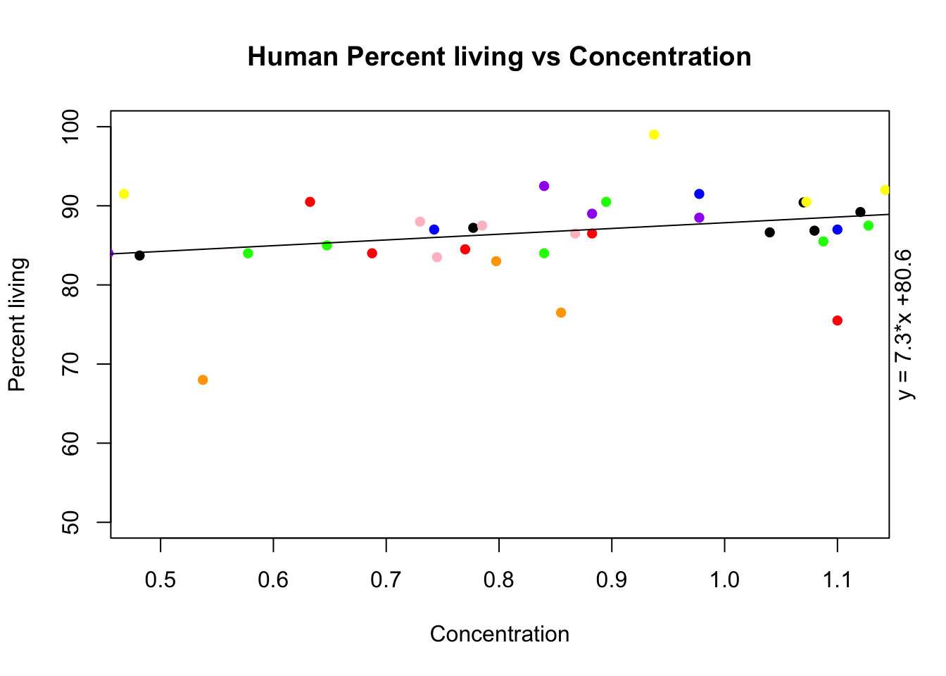
plot(alive_e$avg_c ~ growth_e$avg_c, ylab="Percent living", xlab="Concentration", ylim=c(0,100), pch=16, main="Chimp Percent living vs Concentration")
points(alive_e$c_c3641 ~ growth_e$c_c3641, col="red", pch=16)
points(alive_e$c_pt30 ~ growth_e$c_pt30, col="orange", pch=16)
points(alive_e$c_pt91 ~ growth_e$c_pt91, col="yellow", pch=16)
points(alive_e$c_3610 ~ growth_e$c_3610, col="green", pch=16)
points(alive_e$c_3659 ~ growth_e$c_3659, col="blue", pch=16)
points(alive_e$c_18358 ~ growth_e$c_18358, col="purple", pch=16)
points(alive_e$c_18359 ~ growth_e$c_18359, col="pink", pch=16)
points(alive_e$c_3622 ~ growth_e$c_3622, col="grey", pch=16)
reg= lm(alive_e$avg_c~ growth_e$avg_c)
coeff=coefficients(reg)
eq = paste0("y = ", round(coeff[2],1), "*x +", round(coeff[1],1))
abline(reg)
mtext(eq, side=4)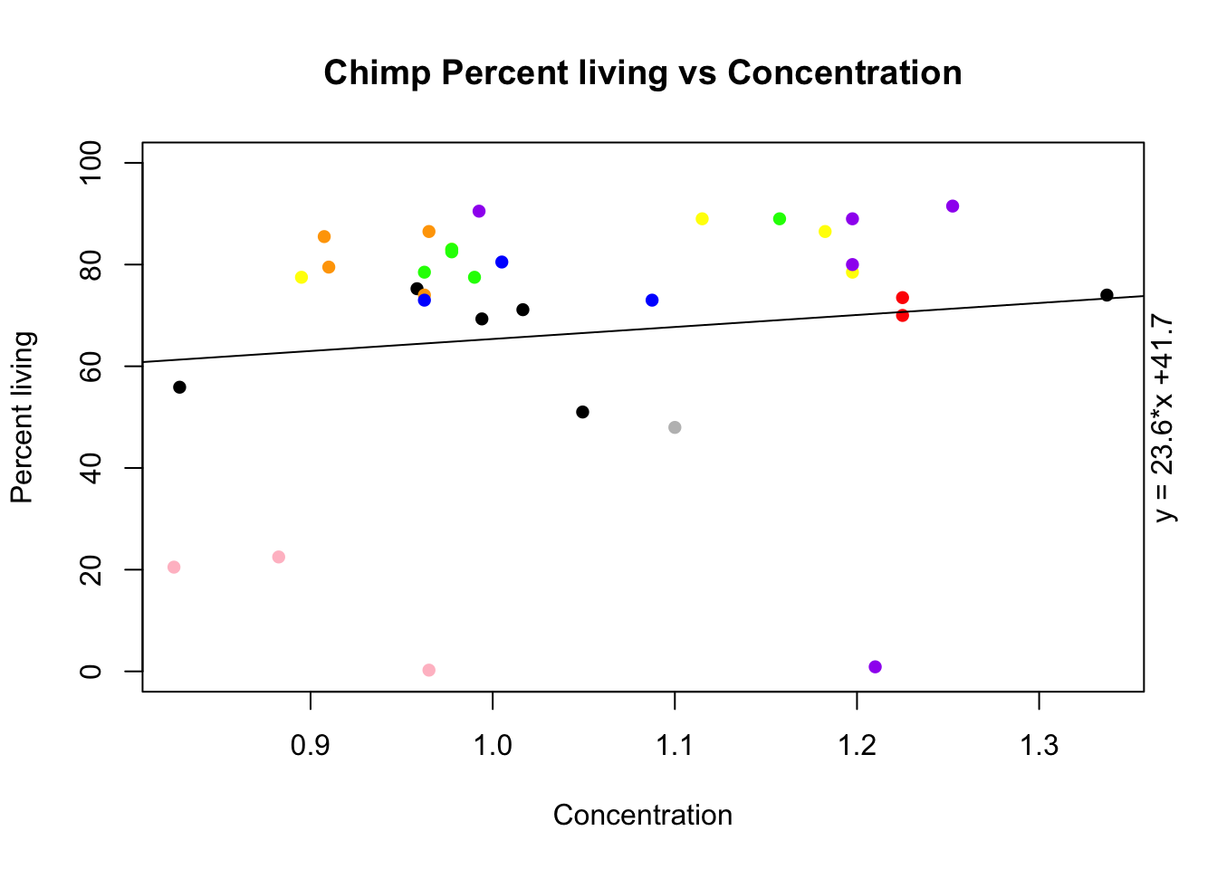 days:
days:
1: saturday
2: sunday
3: monday
4: tuesday
5: wednesday
6: thursday
Before feeding was Feeding happend monday. I will add a verticle line this day.
plot(growth_e$avg_h, xlab="Day", ylim=c(0,2), ylab="cells/ml 10^6", main="Human growth by day")
lines(growth_e$h_18486, col="red")
lines(growth_e$h_18499, col="orange")
lines(growth_e$h_18502, col="yellow")
lines(growth_e$h_18504, col="green")
lines(growth_e$h_18510, col= "blue")
lines(growth_e$h_18517, col="purple")
lines(growth_e$h_18523, col="pink")
abline(v=3, lwd=3, lty=2)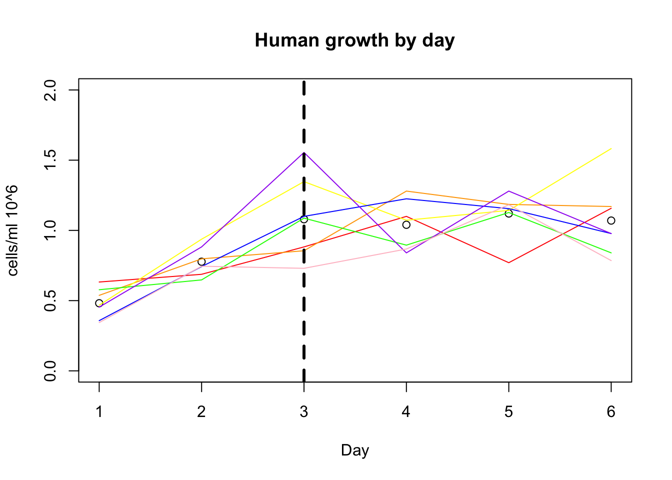
plot(growth_e$avg_c, xlab="Day", ylim=c(0,3), ylab="cells/ml 10^6", main="Chimp Growth by day")
lines(growth_e$c_c3641, col="red")
lines(growth_e$c_pt30, col="orange")
lines(growth_e$c_pt91, col="yellow")
lines(growth_e$c_3610, col="green")
lines(growth_e$c_3659, col= "blue")
lines(growth_e$c_18358, col="purple")
lines(growth_e$c_18359, col="pink")
lines(growth_e$c_3622, col="black")
abline(v=3,lwd=3, lty=2)
add a day post split / feed column so I can plot by this:
days_post=c(1,2,3,1,2,3)
days_post= as.factor(days_post)

growth_e_DP= cbind(days_post,growth_e)
Redo analysis on 3/21
growth_3.21=read.csv("../data/cell_growth_3.21.18.csv", stringsAsFactors = FALSE)

growth_e1=growth_3.21 %>% filter(Type=="e1")

growth_e2=growth_3.21 %>% filter(Type=="e2")
Melt the data:
growth_e2_long=melt(growth_e2, variable.name = "key",value.names = "value", id.vars = c("Line", "Day")) %>% filter(key != "Type")Plot day vs allive:
growth_e2_long_live=growth_e2_long %>% filter(key=="X..Live.average")
ggplot(growth_e2_long, aes(x=as.factor(Day), y=as.numeric(value), group_by(Line)))+ geom_violin()
Warning in fun(x, ...): NAs introduced by coercionWarning in FUN(X[[i]], ...): NAs introduced by coercionWarning: Removed 168 rows containing non-finite values (stat_ydensity).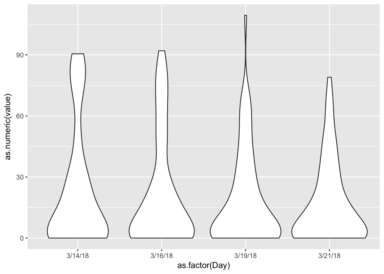
growth_e1_day_group=growth_e1[order(growth_e1$Day),]

growth_e2_day_group=growth_e2[order(growth_e2$Day),]
par(mfrow=c(1,2))
plot(as.factor(growth_e1_day_group$Day),as.numeric(growth_e1_day_group$X..Live.average), main="Percent living by day, E1", ylab="Percent alive" )Warning in is.factor(y): NAs introduced by coercionplot(as.factor(growth_e2_day_group$Day),as.numeric(growth_e2_day_group$X..Live.average), main="Percent living by day, E2", ylab="Percent alive")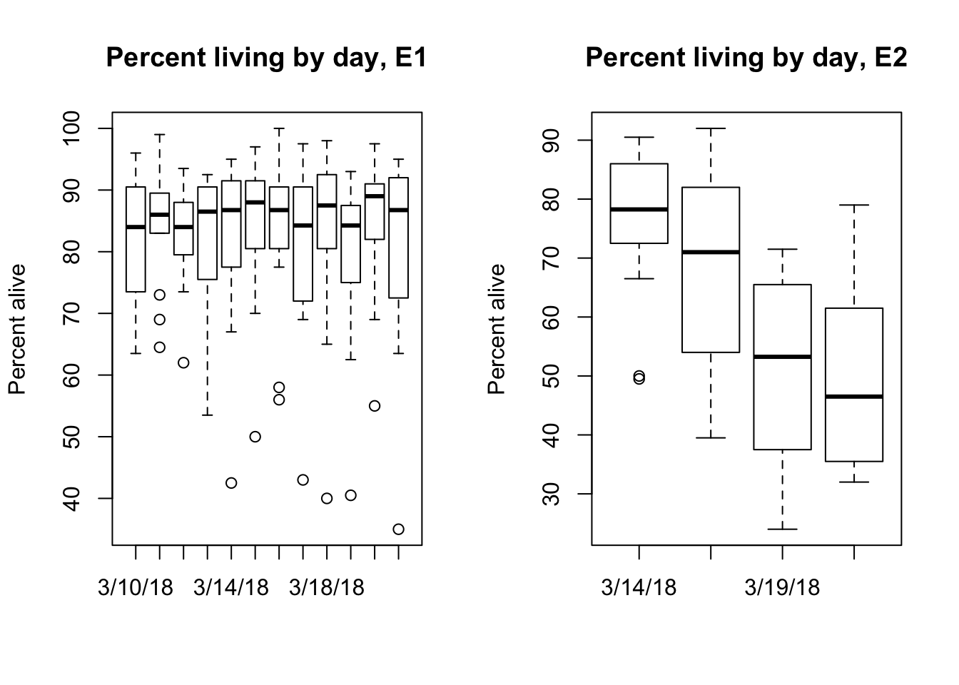
growth_e1_long_av=melt(growth_e1, variable.name = "key",value.names = "value", id.vars = c("Line", "Day")) %>% filter(key=="Average")


ggplot(growth_e1_long_av,aes(x=as.factor(Day), y=as.numeric(value))) + geom_point(aes(col=Line)) + labs(x="Day", y="cells/ml in 10^6") + ggtitle("Cell density")
Warning in fun(x, ...): NAs introduced by coercionWarning in FUN(X[[i]], ...): NAs introduced by coercionWarning: Removed 1 rows containing missing values (geom_point).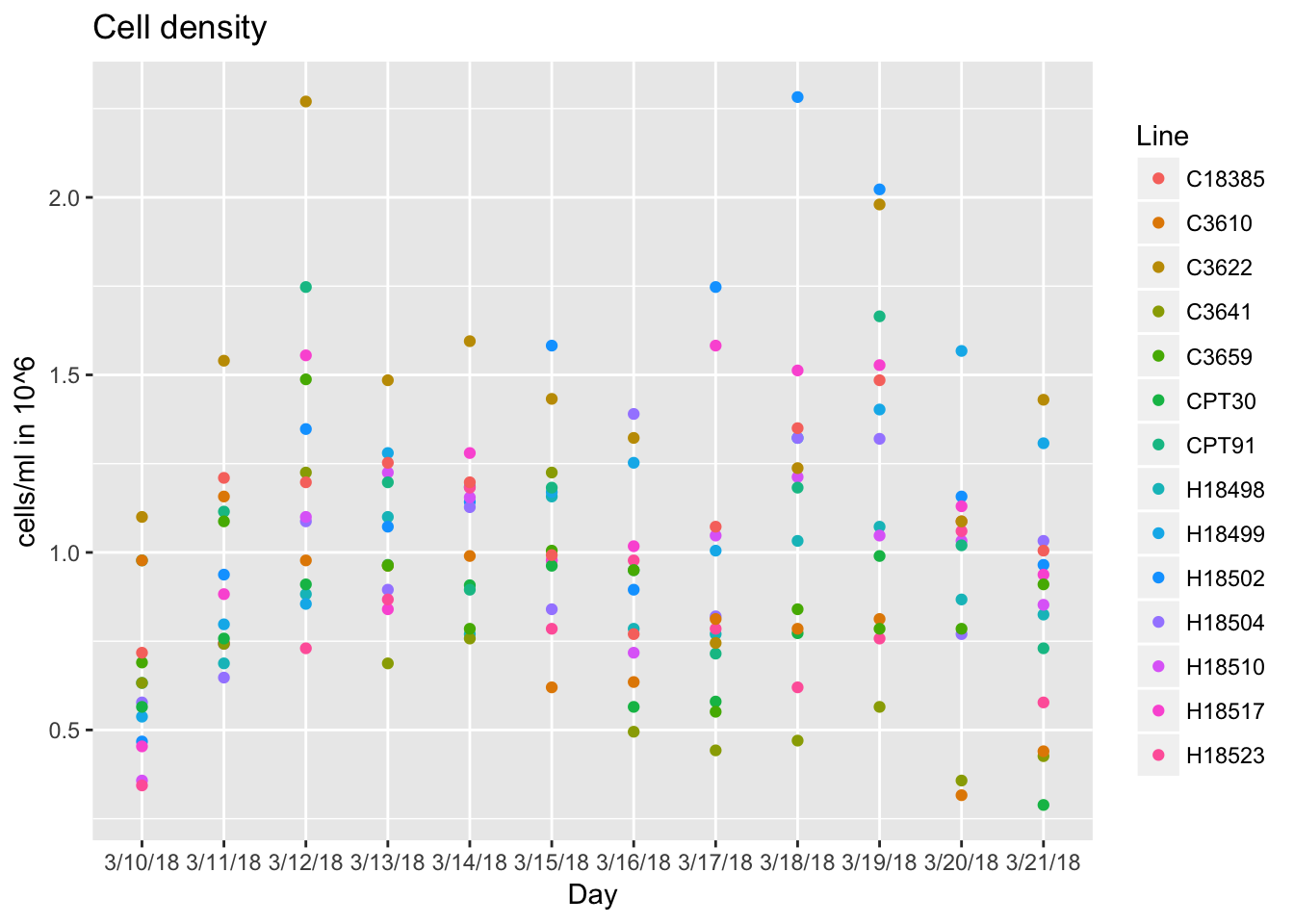
growth_e1_long_live=melt(growth_e1, variable.name = "key",value.names = "value", id.vars = c("Line", "Day")) %>% filter(key=="X..Live.average")


ggplot(growth_e1_long_live,aes(x=as.factor(Day), y=as.numeric(value))) + geom_point(aes(col=Line)) + labs(x="Day", y="Percent Alive") + ggtitle("% Alive by day and line")
Warning in fun(x, ...): NAs introduced by coercionWarning in FUN(X[[i]], ...): NAs introduced by coercionWarning: Removed 1 rows containing missing values (geom_point).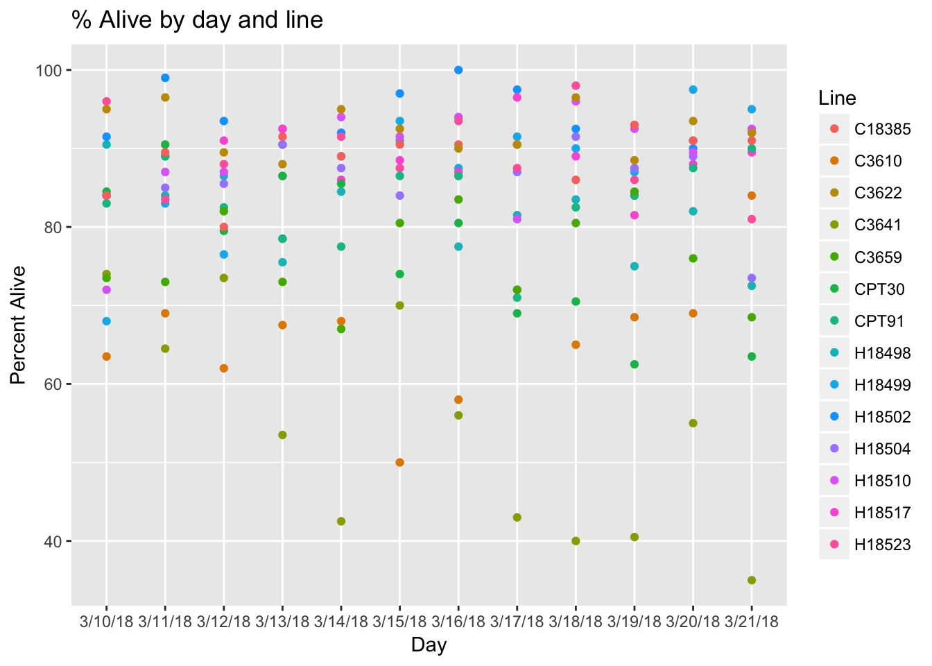
species=c(rep("H", 84), rep("C", 84))
palette(c("red", "blue"))
growth_e1=cbind(growth_e1, species)
plot(as.numeric(growth_e1$Average)~as.numeric(growth_e1$X..Live.average),col=as.factor(growth_e1$species),pch=16, main="Density vs Percent alive", ylab="Cells/ML in 10^6", xlab="Percent Alive")
Warning in eval(predvars, data, env): NAs introduced by coercion
Warning in eval(predvars, data, env): NAs introduced by coercionlegend("topleft", legend=c("Humans", "Chimps"),
col=c("red", "blue"), pch=16, cex=1, title="Species")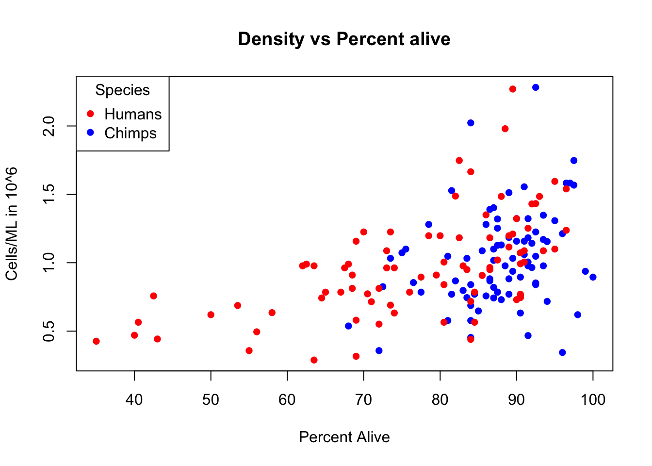
Session information
sessionInfo()R version 3.4.2 (2017-09-28)
Platform: x86_64-apple-darwin15.6.0 (64-bit)
Running under: macOS Sierra 10.12.6
Matrix products: default
BLAS: /Library/Frameworks/R.framework/Versions/3.4/Resources/lib/libRblas.0.dylib
LAPACK: /Library/Frameworks/R.framework/Versions/3.4/Resources/lib/libRlapack.dylib
locale:
[1] en_US.UTF-8/en_US.UTF-8/en_US.UTF-8/C/en_US.UTF-8/en_US.UTF-8
attached base packages:
[1] stats graphics grDevices utils datasets methods base
other attached packages:
[1] bindrcpp_0.2 reshape2_1.4.3 ggplot2_2.2.1 tidyr_0.7.2
[5] dplyr_0.7.4
loaded via a namespace (and not attached):
[1] Rcpp_0.12.15 knitr_1.18 bindr_0.1 magrittr_1.5
[5] munsell_0.4.3 colorspace_1.3-2 R6_2.2.2 rlang_0.1.6
[9] plyr_1.8.4 stringr_1.2.0 tools_3.4.2 grid_3.4.2
[13] gtable_0.2.0 git2r_0.21.0 htmltools_0.3.6 lazyeval_0.2.1
[17] yaml_2.1.16 rprojroot_1.3-2 digest_0.6.14 assertthat_0.2.0
[21] tibble_1.4.2 purrr_0.2.4 glue_1.2.0 evaluate_0.10.1
[25] rmarkdown_1.8.5 labeling_0.3 stringi_1.1.6 compiler_3.4.2
[29] pillar_1.1.0 scales_0.5.0 backports_1.1.2 pkgconfig_2.0.1 This R Markdown site was created with workflowr