Initial Data exploration of Net-3
Briana Mittleman
2018-02-14
Last updated: 2018-02-23
Code version: 4449fa3
Mapped reads
This analysis is to look at the quality of the library net-3. This has the first 8 libraries from the 16 pilot libraries.
18505
18508
18486
19239
19141
19193
19257
19128
The first step is to run the raw reads through my snakefile. To do this I have to change the project directory in the /project2/gilad/briana/net_seq_pipeline/config.yaml to /project2/gilad/briana/Net-seq/Net-seq3/ .
The reads will go in: /project2/gilad/briana/Net-seq/Net-seq3/data/fastq/
I first use gunzip to unzip all of the fastq files then I submit the snakemake file from /project2/gilad/briana/net_seq_pipeline with nohup scripts/submit-snakemake.sh
Look at number of reads, mapped reads, deduplicated reads.
‘samtools view -c -F 4’
libraries=c("18486", "18505", "18508", "19128", "19141", "19193", "19239", '19257')
fastq=c( 34342214,42959246,51413661, 57292491,52841852,60898831,54253650,45506210)
mapped=c(14018943,23607050,26532568,38084941,28165596,37084191,37095436,26636660)
dedup= c(1446379, 1032174,1642314,2469438,1926300,2717515, 2361238, 1377712 )

read_count=rbind(fastq,mapped,dedup)
colnames(read_count)=libraries
total_reads= sum(fastq)
total_reads[1] 399508155total_map= sum(mapped)
total_map[1] 231225385total_dedup= sum(dedup)
total_dedup[1] 14973070total_map/total_reads[1] 0.5787751total_dedup/total_map[1] 0.0647553Make a plot to look at this by line:
count_plot=barplot(as.matrix(read_count), main="Counts for coverage and complexity",
  xlab="Library", col=c("lightskyblue2","dodgerblue1","navy"),
    ylab="Read counts")
legend("topleft", legend = c("total", "mapped", "UMI"), col=c("lightskyblue2","dodgerblue1","navy"), pch=20, cex = .75)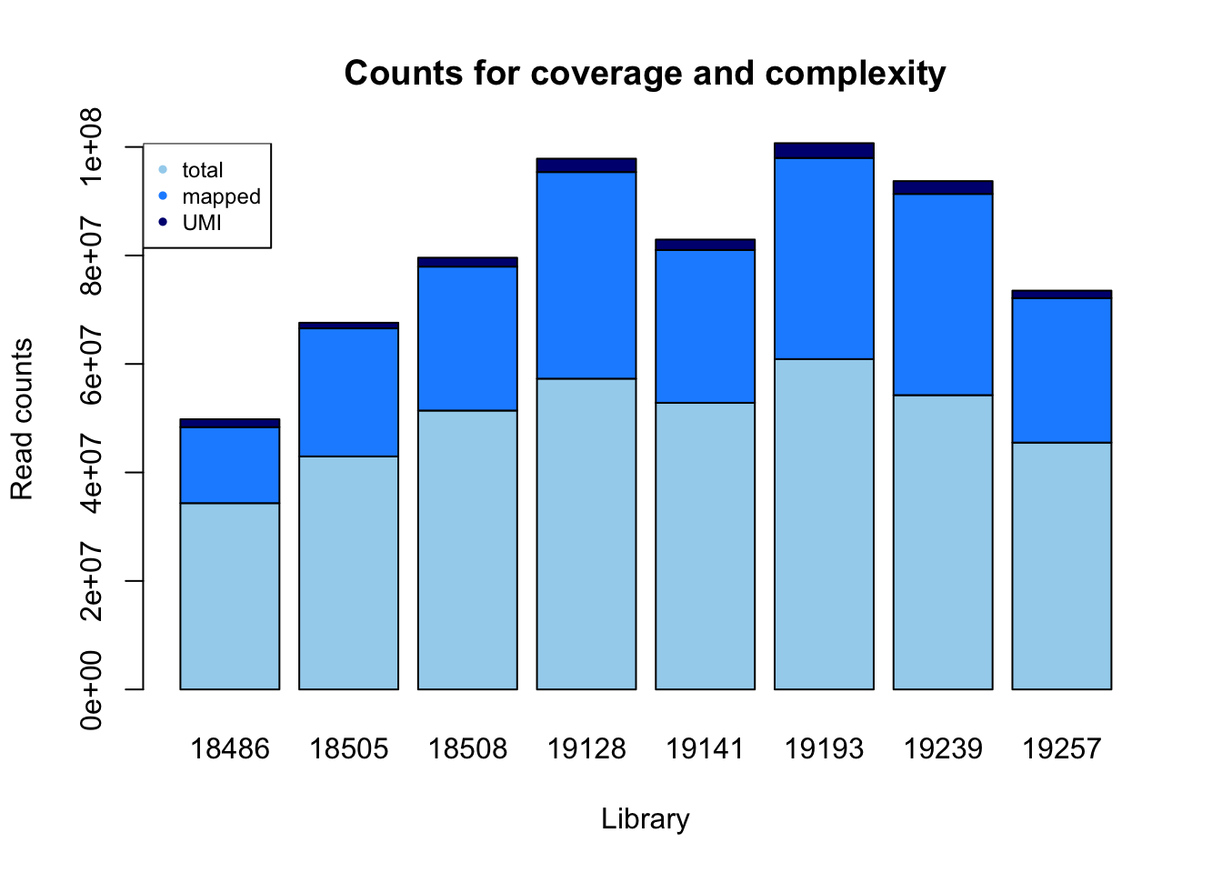
Look at this by proportions:
percent_mapped= mapped/fastq
percent_UMI= dedup/fastq
percent_mapped= percent_mapped - percent_UMI
percent_not_mapped= 1- percent_mapped - percent_UMI


prop=rbind(percent_not_mapped, percent_mapped, percent_UMI)
colnames(prop)= libraries

prop_plot=barplot(as.matrix(prop), main="Proportions for coverage and complexity",
  xlab="Library", col=c("lightskyblue2","dodgerblue1","navy"),
    ylab="Proportion of sequenced reads")
legend("bottomright", legend = c("un-mapped", "mapped", "UMI"), col=c("lightskyblue2","dodgerblue1","navy"), pch=20, cex = 0.75)
summary(mapped) Min. 1st Qu. Median Mean 3rd Qu. Max.
14018943 25801188 27401128 28903173 37087002 38084941 summary(percent_mapped) Min. 1st Qu. Median Mean 3rd Qu. Max.
0.3661 0.4935 0.5403 0.5317 0.5787 0.6402 summary(percent_not_mapped) Min. 1st Qu. Median Mean 3rd Qu. Max.
0.3163 0.3771 0.4326 0.4313 0.4712 0.5918 summary(percent_UMI) Min. 1st Qu. Median Mean 3rd Qu. Max.
0.02403 0.03153 0.03929 0.03701 0.04321 0.04462 percent_mapped[1] 0.3660965 0.5254952 0.4841175 0.6216435 0.4965628 0.5643241 0.6402186
[8] 0.5550660percent_UMI[1] 0.04211665 0.02402682 0.03194314 0.04310230 0.03645406 0.04462343
[7] 0.04352220 0.03027525I will now use the get_mapped.py script from the previous analysis to see how long the mapped reads are. I copied it to /project2/gilad/briana/Net-seq/Net-seq3/code. The code takes in sorted bam file and an output text file. I will create a sbatch script to run this on all 8 files. This file is called wrap_get_mapped.sh and is in the same code directory.
#!/bin/bash


#SBATCH --job-name=wrap_get_map
#SBATCH --time=8:00:00
#SBATCH --partition=gilad
#SBATCH --mem=16G
#SBATCH --mail-type=END

module load Anaconda3

source activate net-seq

python /project2/gilad/briana/Net-seq/Net-seq3/code/get_mapped.py /project2/gilad/briana/Net-seq/Net-seq3/data/sort/YG-SP-NET3-18486-2018-1-8_S3_L008_R1_001-sort.bam /project2/gilad/briana/Net-seq/Net-seq3/output/mapped_stats_18486.txt

python /project2/gilad/briana/Net-seq/Net-seq3/code/get_mapped.py /project2/gilad/briana/Net-seq/Net-seq3/data/sort/YG-SP-NET3-18505-2018-1-8_S1_L008_R1_001-sort.bam /project2/gilad/briana/Net-seq/Net-seq3/output/mapped_stats_18505.txt

python /project2/gilad/briana/Net-seq/Net-seq3/code/get_mapped.py /project2/gilad/briana/Net-seq/Net-seq3/data/sort/YG-SP-NET3-18508-2018-1-8_S2_L008_R1_001-sort.bam /project2/gilad/briana/Net-seq/Net-seq3/output/mapped_stats_18508.txt

python /project2/gilad/briana/Net-seq/Net-seq3/code/get_mapped.py /project2/gilad/briana/Net-seq/Net-seq3/data/sort/YG-SP-NET3-19128-2018-1-8_S8_L008_R1_001-sort.bam /project2/gilad/briana/Net-seq/Net-seq3/output/mapped_stats_19128.txt


python /project2/gilad/briana/Net-seq/Net-seq3/code/get_mapped.py /project2/gilad/briana/Net-seq/Net-seq3/data/sort/YG-SP-NET3-19141-2018-1-8_S5_L008_R1_001-sort.bam /project2/gilad/briana/Net-seq/Net-seq3/output/mapped_stats_19141.txt

python /project2/gilad/briana/Net-seq/Net-seq3/code/get_mapped.py /project2/gilad/briana/Net-seq/Net-seq3/data/sort/YG-SP-NET3-19193-2018-1-8_S6_L008_R1_001-sort.bam /project2/gilad/briana/Net-seq/Net-seq3/output/mapped_stats_19193.txt

python /project2/gilad/briana/Net-seq/Net-seq3/code/get_mapped.py /project2/gilad/briana/Net-seq/Net-seq3/data/sort/YG-SP-NET3-19239-2018-1-8_S4_L008_R1_001-sort.bam /project2/gilad/briana/Net-seq/Net-seq3/output/mapped_stats_19239.txt

python /project2/gilad/briana/Net-seq/Net-seq3/code/get_mapped.py /project2/gilad/briana/Net-seq/Net-seq3/data/sort/YG-SP-NET3-19257-2018-1-8_S7_L008_R1_001-sort.bam /project2/gilad/briana/Net-seq/Net-seq3/output/mapped_stats_19257.txt
I will now make histograms showing the number of reads that map from the cigar strings.
#pull in data:

map.vec.18486=read.csv("../data/net-3-readmap/mapped_stats_18486.txt", header=FALSE)
map.vec.18505=read.csv("../data/net-3-readmap/mapped_stats_18505.txt", header=FALSE)
map.vec.18508=read.csv("../data/net-3-readmap/mapped_stats_18508.txt", header=FALSE)
map.vec.19128=read.csv("../data/net-3-readmap/mapped_stats_19128.txt", header=FALSE)
map.vec.19141=read.csv("../data/net-3-readmap/mapped_stats_19141.txt", header=FALSE)
map.vec.19193=read.csv("../data/net-3-readmap/mapped_stats_19193.txt", header=FALSE)
map.vec.19239=read.csv("../data/net-3-readmap/mapped_stats_19239.txt", header=FALSE)
map.vec.19257=read.csv("../data/net-3-readmap/mapped_stats_19257.txt", header=FALSE)
#pull in mayer as well

map.vec.mayer=read.csv("../data/mapped_mayer.txt", header=FALSE)
#make histograms
par(mfrow=c(3,3))
hist((as.numeric(map.vec.18486$V1)), xlab="Bases", main="Histogram of 18486 mapped reads")
hist((as.numeric(map.vec.18505$V1)), xlab="Bases", main="Histogram of 18505 mapped reads")
hist((as.numeric(map.vec.18508$V1)), xlab="Bases", main="Histogram of 18508 mapped reads")
hist((as.numeric(map.vec.19128$V1)), xlab="Bases", main="Histogram of 19128 mapped reads")
hist((as.numeric(map.vec.19141$V1)), xlab="Bases", main="Histogram of 19141 mapped reads")
hist((as.numeric(map.vec.19193$V1)), xlab="Bases", main="Histogram of 19193 mapped reads")
hist((as.numeric(map.vec.19239$V1)), xlab="Bases", main="Histogram of 19239 mapped reads")
hist((as.numeric(map.vec.19257$V1)), xlab="Bases", main="Histogram of 19257 mapped reads")
hist((as.numeric(map.vec.mayer$V1)), xlab="Bases", main="Histogram of Mayer mapped reads")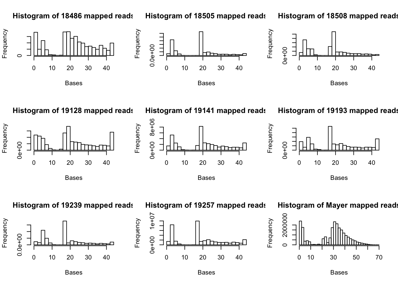
Deep tools analysis:
First I downloaded the gencode.hg19 gene gtf file. I will use bedops convert2bed.
awk '{ if ($0 ~ "transcript_id") print $0; else print $0" transcript_id \"\";"; }' gencode.v19.annotation.gtf | gtf2bed - > gencode.v19.annotation.bed
Deep tools code:
#!/bin/bash


#SBATCH --job-name=deeptools_netseq
#SBATCH --time=8:00:00
#SBATCH --partition=broadwl
#SBATCH --mem=30G
#SBATCH --mail-type=END
#SBATCH --output=deeptool_sbatch.out
#SBATCH --error=deeptools_sbatch.err

module load Anaconda3

source activate net-seq

bamCoverage -b /project2/gilad/briana/Net-seq/Net-seq3/data/sort/YG-SP-NET3-18486-2018-1-8_S3_L008_R1_001-sort.bam -o /project2/gilad/briana/Net-seq/Net-seq3/output/deeptools/net-seq-18486.bw

computeMatrix reference-point -S /project2/gilad/briana/Net-seq/Net-seq3/output/deeptools/net-seq-18486.bw -R /project2/gilad/briana/Net-seq/Net-seq3/gencode.v19.annotation.bed --referencePoint TSS -b 100 -a 100 -out /project2/gilad/briana/Net-seq/Net-seq3/output/deeptools/net-seq-18486.gz

plotHeatmap --sortRegions descend --refPointLabel "TSS" -m /project2/gilad/briana/Net-seq/Net-seq3/output/deeptools/net-seq-18486.gz  -out /project2/gilad/briana/Net-seq/Net-seq3/output/deeptools/net-seq-18486.png
To look at TES I will change the reference point to TES. This script is also in the code file as deep_tools_TES_net18486.sh.
#!/bin/bash


#SBATCH --job-name=deeptools_TES_netseq
#SBATCH --time=8:00:00
#SBATCH --partition=broadwl
#SBATCH --mem=30G
#SBATCH --mail-type=END
#SBATCH --output=deeptool_TES_sbatch.out
#SBATCH --error=deeptools_TES_sbatch.err

module load Anaconda3

source activate net-seq

#the bw file has already been created

computeMatrix reference-point -S /project2/gilad/briana/Net-seq/Net-seq3/output/deeptools/net-seq-18486.bw -R /project2/gilad/briana/Net-seq/Net-seq3/gencode.v19.annotation.bed --referencePoint TES -b 100o -a 1000 -out /project2/gilad/briana/Net-seq/Net-seq3/output/deeptools/net-seq-TES-18486.gz

plotHeatmap --sortRegions descend --refPointLabel "TSS"  -m /project2/gilad/briana/Net-seq/Net-seq3/output/deeptools/net-seq-TES-18486.gz  -out /project2/gilad/briana/Net-seq/Net-seq3/output/deeptools/net-seq-TES-18486.png
Do this for DNA hypersensitivity clusters as well. This script is in the code file as deep_tools_DHS_net18486.sh.
#!/bin/bash


#SBATCH --job-name=deeptools_DHS_netseq
#SBATCH --time=8:00:00
#SBATCH --partition=broadwl
#SBATCH --mem=30G
#SBATCH --mail-type=END
#SBATCH --output=deeptool_DHS_sbatch.out
#SBATCH --error=deeptools_DHS_sbatch.err

module load Anaconda3

source activate net-seq

#the bw file has already been created

computeMatrix reference-point -S /project2/gilad/briana/Net-seq/Net-seq3/output/deeptools/net-seq-18486.bw -R /project2/gilad/briana/Net-seq/Net-seq3/wgEncodeRegDnaseClusteredV3.bed -b 1000 -a 1000 -out /project2/gilad/briana/Net-seq/Net-seq3/output/deeptools/net-seq-dhs-18486.gz

plotHeatmap --sortRegions descend --refPointLabel "DHS" -m /project2/gilad/briana/Net-seq/Net-seq3/output/deeptools/net-seq-dhs-18486.gz  -out /project2/gilad/briana/Net-seq/Net-seq3/output/deeptools/net-seq-dhs-18486.png
I am running these and 1 more looking at the TSS but at 1000 base pairs on each side.
timed out at 1000 need to try 500 on each side
Gene counts with Feature counts
I will use featureCounts to count the number of reads at each gene in the gencode.v19.annotation.gtf file. I will make a file that takes the bam as a input so I can run it on each bam file.
‘Usage: featureCounts [options] -a
This file is in the net3 code directory. featureCounts_genes.sh
#!/bin/bash


#SBATCH --job-name=featureCounts
#SBATCH --time=8:00:00
#SBATCH --partition=broadwl
#SBATCH --mem=16G
#SBATCH --mail-type=END
#SBATCH --output=featurecount.out
#SBATCH --error=featurecount.err


#$1 input bam full file

module load Anaconda3

source activate net-seq


sample=$1


describer=$(echo ${sample} | sed -e 's/.*\YG-SP-//' | sed -e "s/_L008_R1_001-sort.bam$//")


featureCounts -a /project2/gilad/briana/Net-seq/Net-seq3/gencode.v19.annotation.gtf -o /project2/gilad/briana/Net-seq/Net-seq3/output/featureCounts/${sample}-gene-counts.txt ${sample}
Try this with one file. /project2/gilad/briana/Net-seq/Net-seq3/data/sort/YG-SP-NET3-18486-2018-1-8_S3_L008_R1_001-sort.bam
Bedtools coverage is a better program for this analyisis. I want to look at coverage along the full gene, not by exon/transcript.
Need to cut the chr from the gencode file so this matches the way my bam files are written. cat gencode.Genes.bed |sed 's/^chr//' > gencode_noCHR_genes.bed
This is in the code directory as gencode_cov.sh
#!/bin/bash


#SBATCH --job-name=count_cov
#SBATCH --output=count_cov_sbatch.out
#SBATCH --error=count_cov_sbatch.err
#SBATCH --time=8:00:00
#SBATCH --partition=broadwl
#SBATCH --mem=36G
#SBATCH --mail-type=END

module load Anaconda3

source activate net-seq


sample=$1

describer=$(echo ${sample} | sed -e 's/.*\YG-SP-//' | sed -e "s/_L008_R1_001-sort.bam$//")

bedtools coverage -counts -sorted -a /project2/gilad/briana/Net-seq/Net-seq3/gencode_noCHR_genes_MT_Fsort.bed -b $1 > /project2/gilad/briana/Net-seq/Net-seq3/data/gencode_cov/${describer}.coverage.bed
run on /project2/gilad/briana/Net-seq/Net-seq3/data/sort/YG-SP-NET3-18486-2018-1-8_S3_L008_R1_001-sort.bam
I will run this on all 8 files then merge the files.
To merge:
touch all_files_coverage.bed
awk '{print $7}' NET3-18486-2018-1-8_S3.coverage.bed | paste -d'' all_files_coverage.bed  > all_files_coverage.bed


cp all_files_coverage.bed tmp
for i in `cat list_of_files.txt`; do awk 'NR==FNR {a[NR]=$7;next} {print $0,a[FNR]}' $i tmp > tmp2; mv tmp2 tmp; done

cut -f -6  NET3-18486-2018-1-8_S3.coverage.bed > meta_info_coverage.bed
Now I will have the meta data seperate from the matrix of counts.
net_coverage=read.table("../data/all_files_coverage.bed", header=FALSE)
colnames(net_coverage)= libraries
net_coverage_meta=read.table("../data/meta_info_coverage.bed", header=FALSE)
colnames(net_coverage_meta)=c("chr", "start", "end", "gene", "score", "strand")
Make one with counts and meta info:
net_cov_full= cbind(net_coverage_meta, net_coverage)Make a function that will tell me proportion of genes detected.
genes_detected=function(col){
  #takes in net_cov_full col which corresponds to one library
  tot_genes=nrow(net_cov_full)
  exp_genes=sum(col!=0)
  return(exp_genes/tot_genes)
}

prop_non0= c(genes_detected(net_cov_full$`18486`), genes_detected(net_cov_full$`18505`),genes_detected(net_cov_full$`18508`), genes_detected(net_cov_full$`19128`), genes_detected(net_cov_full$`19141`), genes_detected(net_cov_full$`19193`), genes_detected(net_cov_full$`19239`), genes_detected(net_cov_full$`19257`))
names(prop_non0)=libraries

barplot(prop_non0, ylim = c(0,1), main="Net-seq Genes detected", ylab="Proportion non zero genes", xlab="Library", col = 'Blue')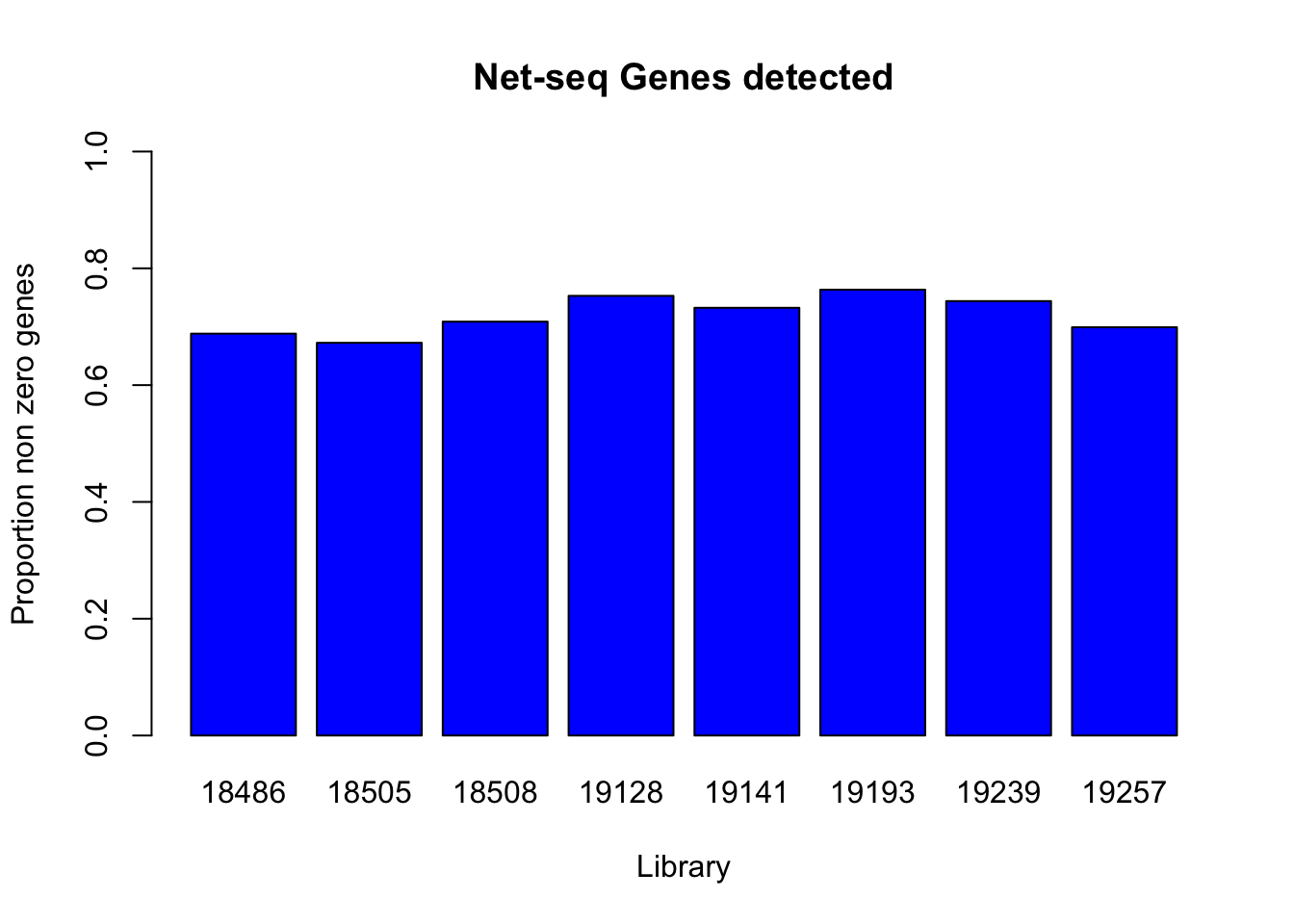
Heatmap to see relatedness:
cor_function=function(data){
  corr_matrix= matrix(0,8,8)
  for (i in seq(1,8)){
    for (j in seq(1,8)){
      x=cor.test(net_coverage[,i],  net_coverage[,j], method='pearson')
      cor_ij=as.numeric(x$estimate)
      corr_matrix[i,j]=cor_ij
    }
  }
  return(corr_matrix)
}


net_cor_matrix=cor_function(net_coverage)
rownames(net_cor_matrix)=c("NA18486", "NA18505", "NA18508", "NA19128", "NA19141", "NA19193", "NA19239", 'NA19257')
colnames(net_cor_matrix)=c("NA18486", "NA18505", "NA18508", "NA19128", "NA19141", "NA19193", "NA19239", 'NA19257')library(reshape2)Warning: package 'reshape2' was built under R version 3.4.3library(ggplot2)
melted_net_corr=melt(net_cor_matrix)
head(melted_net_corr) Var1 Var2 value
1 NA18486 NA18486 1.0000000
2 NA18505 NA18486 0.9555217
3 NA18508 NA18486 0.9526759
4 NA19128 NA18486 0.9799010
5 NA19141 NA18486 0.9822975
6 NA19193 NA18486 0.9699379ggheatmap=ggplot(data = melted_net_corr, aes(x=Var1, y=Var2, fill=value)) +
geom_tile() +
labs(title="Net-seq Correlation Heatplot")
ggheatmap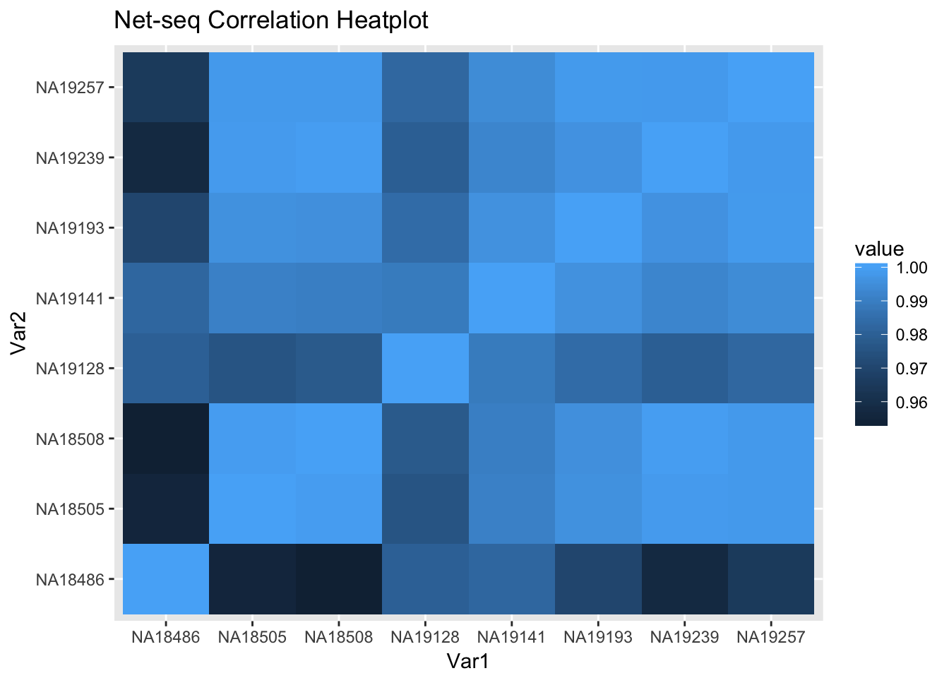
Look at the distribution of read counts:
- Create a length of gene column to standardize by length.
summary(net_cov_full$`18486`) Min. 1st Qu. Median Mean 3rd Qu. Max.
0.0 0.0 5.0 325.7 22.0 2651806.0 plot(log10(sort(net_cov_full$`18486`, decreasing = TRUE)))
plot(log(sort(net_cov_full$`18505`, decreasing = TRUE)))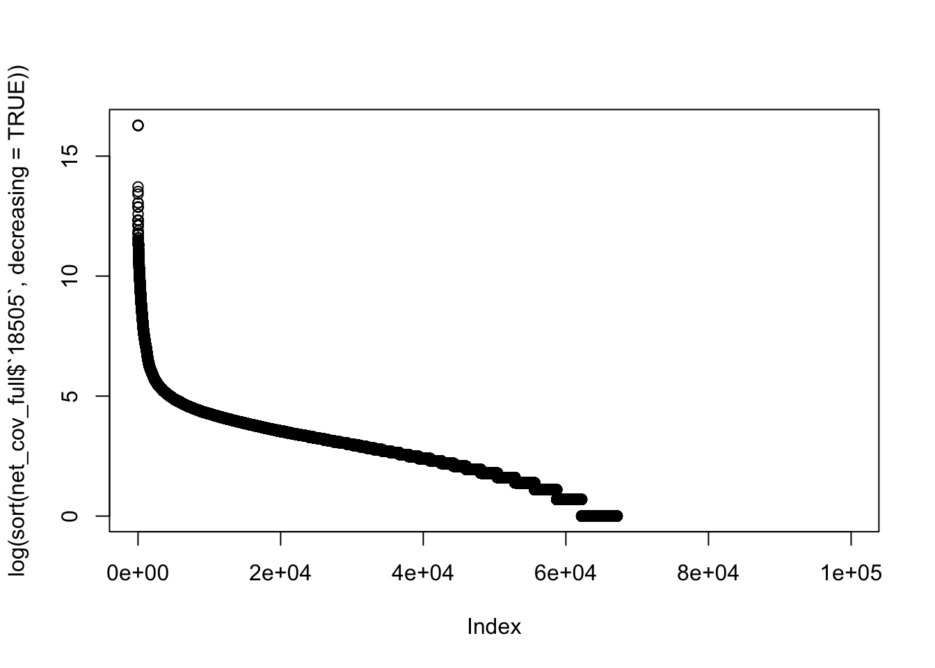
which(net_cov_full$`18486`== max(net_cov_full$`18486`))[1] 12688 12689net_cov_full[12688,] chr start end gene score strand 18486
12688 2 118846049 118867604 ENST00000245787.4 0 + 2651806
18505 18508 19128 19141 19193 19239 19257
12688 11856396 14059279 10862066 8216975 11877635 18071447 10156398which(net_cov_full$`19239`== max(net_cov_full$`19239`))[1] 12689net_cov_full[12689,] chr start end gene score strand 18486
12689 2 118846049 118868573 ENST00000485520.1 0 + 2651806
18505 18508 19128 19141 19193 19239 19257
12689 11856396 14059279 10862067 8216975 11877635 18071449 10156398read buildup in insig2!
To look into this I will use bedtools genomecov. This will help me find the region where the build up is within this gene. I will do this for just one line first.
‘bedtools genomecov -ibam NA18152.bam -bg’
#!/bin/bash


#SBATCH --job-name=gencov_18486
#SBATCH --time=8:00:00
#SBATCH --partition=broadwl
#SBATCH --mem=20G
#SBATCH --output=gencov_sbatch.out
#SBATCH --error=gencov_sbatch.err
#SBATCH --mail-type=END

module load Anaconda3

source activate net-seq


bedtools genomecov -ibam /project2/gilad/briana/Net-seq/Net-seq3/data/sort/YG-SP-NET3-18486-2018-1-8_S3_L008_R1_001-sort.bam -bg
I made this file, now I can look for the region and find the base position of the buildup.
gencov_18486=read.csv("../data/gencov_18486.bed", header=FALSE, sep = "\t", stringsAsFactors = FALSE)
colnames(gencov_18486)=c("chr", "start", "end", "count")


gencov_18486_insig2= gencov_18486[gencov_18486$chr == "2" & gencov_18486$start >= 118846049 & gencov_18486$end <= 118868573, ]
Buildup is 118847163-118867371
https://genome.ucsc.edu/cgi-bin/hgTracks?db=hg19&lastVirtModeType=default&lastVirtModeExtraState=&virtModeType=default&virtMode=0&nonVirtPosition=&position=chr2%3A118853899%2D118860634&hgsid=657371987_p3YvC1JmckcMJLpbqv6SsBjfPeik
http://genome.ucsc.edu/cgi-bin/das/hg19/dna?segment=chr2:118847163,118867371I will now be able to search for our primers in this seq to see if that is why we get buildup.
GACGCTCTT
This sequence is in the reverse compliment of the linker:
/5rApp/(N)6AGATCGGAAGAGCGTC/3ddC
This is probably not long enough that this is the problem.
Mapping statistics:
The quality score is in the sorted bam file.
MAPQ: MAPping Quality. It equals -10*log10 Prob mapping position is wrong, rounded to the nearest integer. A value 255 indicates that the mapping quality is not available.
I will get the mapping quality stats from the bam files as I did for Net1. I coppied the pytho script to /project2/gilad/briana/Net-seq/Net-seq3/code. I will create a wrap function for this in bash.
#!/bin/bash


#SBATCH --job-name=wrap_get_map
#SBATCH --time=8:00:00
#SBATCH --partition=broadwl
#SBATCH --mem=20G
#SBATCH --mail-type=END

module load Anaconda3

source activate net-seq

python /project2/gilad/briana/Net-seq/Net-seq3/code/get_qual.py /project2/gilad/briana/Net-seq/Net-seq3/data/sort/YG-SP-NET3-18486-2018-1-8_S3_L008_R1_001-sort.bam /project2/gilad/briana/Net-seq/Net-seq3/output/mapped_qual_18486.txt

python /project2/gilad/briana/Net-seq/Net-seq3/code/get_qual.py /project2/gilad/briana/Net-seq/Net-seq3/data/sort/YG-SP-NET3-18505-2018-1-8_S1_L008_R1_001-sort.bam /project2/gilad/briana/Net-seq/Net-seq3/output/mapped_qual_18505.txt

python /project2/gilad/briana/Net-seq/Net-seq3/code/get_qual.py /project2/gilad/briana/Net-seq/Net-seq3/data/sort/YG-SP-NET3-18508-2018-1-8_S2_L008_R1_001-sort.bam /project2/gilad/briana/Net-seq/Net-seq3/output/mapped_qual_18508.txt

python /project2/gilad/briana/Net-seq/Net-seq3/code/get_qual.py /project2/gilad/briana/Net-seq/Net-seq3/data/sort/YG-SP-NET3-19128-2018-1-8_S8_L008_R1_001-sort.bam /project2/gilad/briana/Net-seq/Net-seq3/output/mapped_qual_19128.txt

python /project2/gilad/briana/Net-seq/Net-seq3/code/get_qual.py /project2/gilad/briana/Net-seq/Net-seq3/data/sort/YG-SP-NET3-19141-2018-1-8_S5_L008_R1_001-sort.bam /project2/gilad/briana/Net-seq/Net-seq3/output/mapped_qual_19141.txt

python /project2/gilad/briana/Net-seq/Net-seq3/code/get_qual.py /project2/gilad/briana/Net-seq/Net-seq3/data/sort/YG-SP-NET3-19193-2018-1-8_S6_L008_R1_001-sort.bam /project2/gilad/briana/Net-seq/Net-seq3/output/mapped_qual_19193.txt

python /project2/gilad/briana/Net-seq/Net-seq3/code/get_qual.py /project2/gilad/briana/Net-seq/Net-seq3/data/sort/YG-SP-NET3-19239-2018-1-8_S4_L008_R1_001-sort.bam /project2/gilad/briana/Net-seq/Net-seq3/output/mapped_qual_19239.txt

python /project2/gilad/briana/Net-seq/Net-seq3/code/get_qual.py /project2/gilad/briana/Net-seq/Net-seq3/data/sort/YG-SP-NET3-19257-2018-1-8_S7_L008_R1_001-sort.bam /project2/gilad/briana/Net-seq/Net-seq3/output/mapped_qual_19257.txt
qual_mayer= read.csv("../data/qual_mayer.txt", head=FALSE)
summary(qual_mayer)
V1
Min. : 6.00
1st Qu.:10.00
Median :13.00
Mean :21.11
3rd Qu.:40.00
Max. :40.00 I will compare our lines to the mayer data.
 mq_18486= read.csv("../data/mapped_qual_18486.txt", header=FALSE)
 mq_18505= read.csv("../data/mapped_qual_18505.txt", header=FALSE)
 mq_18508= read.csv("../data/mapped_qual_18508.txt", header=FALSE)
 mq_19128=read.csv("../data/mapped_qual_19128.txt", header=FALSE)
 mq_19141=read.csv("../data/mapped_qual_19141.txt", header=FALSE)
 mq_19193=read.csv("../data/mapped_qual_19193.txt", header=FALSE)
 mq_19239=read.csv("../data/mapped_qual_19239.txt", header=FALSE)
 mq_19257=read.csv("../data/mapped_qual_19257.txt", header=FALSE)
summaries of each:
summary(mq_18486) V1
Min. : 6.00
1st Qu.:10.00
Median :13.00
Mean :17.46
3rd Qu.:20.00
Max. :40.00 summary(mq_18505) V1
Min. : 6.00
1st Qu.:10.00
Median :10.00
Mean :14.41
3rd Qu.:13.00
Max. :40.00 summary(mq_18508) V1
Min. : 6.00
1st Qu.:10.00
Median :10.00
Mean :14.11
3rd Qu.:13.00
Max. :40.00 summary(mq_19128) V1
Min. : 6.00
1st Qu.:10.00
Median :13.00
Mean :18.75
3rd Qu.:20.00
Max. :40.00 summary(mq_19141) V1
Min. : 6.00
1st Qu.:10.00
Median :13.00
Mean :17.39
3rd Qu.:20.00
Max. :40.00 summary(mq_19193) V1
Min. : 6.00
1st Qu.:10.00
Median :13.00
Mean :18.42
3rd Qu.:20.00
Max. :40.00 summary(mq_19239) V1
Min. : 6.0
1st Qu.:10.0
Median :13.0
Mean :16.3
3rd Qu.:20.0
Max. :40.0 summary(mq_19257) V1
Min. : 6.00
1st Qu.:13.00
Median :13.00
Mean :18.45
3rd Qu.:20.00
Max. :40.00 Make histograms as I had for the net1.
par(mfrow = c(3,3))

hist(as.numeric(mq_18486[,1]), freq=FALSE, main="Quality 18486", xlab="Quality Score")
hist(as.numeric(mq_18505[,1]), freq=FALSE, main="Quality 18505", xlab="Quality Score")
hist(as.numeric(mq_18508[,1]), freq=FALSE, main="Quality 18508", xlab="Quality Score")
hist(as.numeric(mq_19128[,1]), freq=FALSE, main="Quality 19128", xlab="Quality Score")
hist(as.numeric(mq_19141[,1]), freq=FALSE, main="Quality 19141", xlab="Quality Score")
hist(as.numeric(mq_19193[,1]), freq=FALSE, main="Quality 19193", xlab="Quality Score")
hist(as.numeric(mq_19239[,1]), freq=FALSE, main="Quality 19239", xlab="Quality Score")
hist(as.numeric(mq_19257[,1]), freq=FALSE, main="Quality 19257", xlab="Quality Score")
hist(as.numeric(qual_mayer[,1]), freq=FALSE, main= "Quality Mayer", xlab="Quality Score")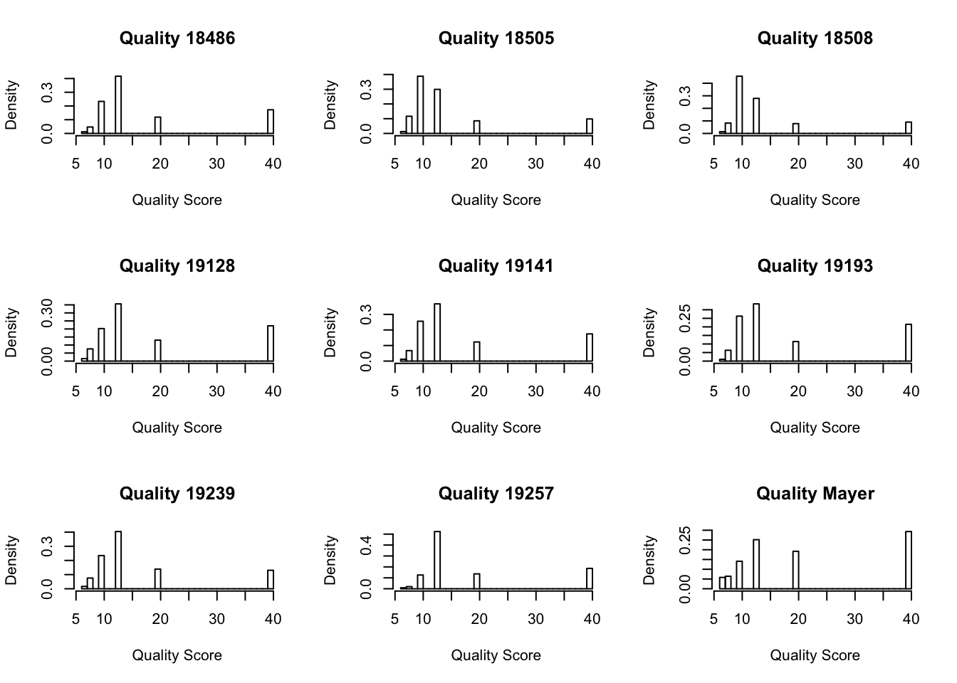
Assess UMI usage:
samtools view YG-SP-NET3-18486-2018-1-8_S3_L008_R1_001-sort.bam  | tr "_" "\t" | cut -f 2 | sort | uniq -c > ../../output/UMI_Net3_18486_stat.txt

samtools view YG-SP-NET3-18505-2018-1-8_S1_L008_R1_001-sort.bam  | tr "_" "\t" | cut -f 2 | sort | uniq -c > ../../output/UMI_18505_stat.txt

samtools view YG-SP-NET3-18508-2018-1-8_S2_L008_R1_001-sort.bam | tr "_" "\t" | cut -f 2 | sort | uniq -c > ../../output/UMI_Net3_18508_stat.txt

samtools view YG-SP-NET3-19128-2018-1-8_S8_L008_R1_001-sort.bam | tr "_" "\t" | cut -f 2 | sort | uniq -c > ../../output/UMI_Net3_19128_stat.txt


samtools view YG-SP-NET3-19141-2018-1-8_S5_L008_R1_001-sort.bam  | tr "_" "\t" | cut -f 2 | sort | uniq -c > ../../output/UMI_Net3_19141_stat.txt


samtools view YG-SP-NET3-19193-2018-1-8_S6_L008_R1_001-sort.bam | tr "_" "\t" | cut -f 2 | sort | uniq -c > ../../output/UMI_Net3_19193_stat.txt

samtools view YG-SP-NET3-19239-2018-1-8_S4_L008_R1_001-sort.bam  | tr "_" "\t" | cut -f 2 | sort | uniq -c > ../../output/UMI_Net3_19239_stat.txt

samtools view YG-SP-NET3-19257-2018-1-8_S7_L008_R1_001-sort.bam | tr "_" "\t" | cut -f 2 | sort | uniq -c > ../../output/UMI_Net3_19257_stat.txt
Function to get the information I want.
library("tidyr")
Attaching package: 'tidyr'The following object is masked from 'package:reshape2':
smithslibrary("dplyr")
Attaching package: 'dplyr'The following objects are masked from 'package:stats':
filter, lagThe following objects are masked from 'package:base':
intersect, setdiff, setequal, unionlibrary("ggplot2")
prepare_UMI_data=function(path.txt){
x=read.delim(file=path.txt, header = FALSE,stringsAsFactors = FALSE)
colnames(x) <- "UMI"
x= data.frame(sapply(x, trimws), stringsAsFactors = FALSE)
x= separate(data=x, col = UMI, into= c("number", "umi"), sep="\\s+")
x$number= as.numeric(x$number)
x= arrange(x, desc(number))
return(x)
}Run function for each file:
UMI_mayer= prepare_UMI_data("../data/UMI_mayer_stat.txt")
UMI_net3_18486= prepare_UMI_data("../data/UMI_Net3_18486_stat.txt")
UMI_net3_18505= prepare_UMI_data("../data/UMI_Net3_18505_stat.txt")
UMI_net3_18508= prepare_UMI_data("../data/UMI_Net3_18508_stat.txt")
UMI_net3_19128= prepare_UMI_data("../data/UMI_Net3_19128_stat.txt")
UMI_net3_19141= prepare_UMI_data("../data/UMI_Net3_19141_stat.txt")
UMI_net3_19193= prepare_UMI_data("../data/UMI_Net3_19193_stat.txt")
UMI_net3_19239= prepare_UMI_data("../data/UMI_Net3_19239_stat.txt")
UMI_net3_19257= prepare_UMI_data("../data/UMI_Net3_19257_stat.txt")
UMI distributions:
par(mfrow = c(3,3))
plot(UMI_net3_18486$number, ylab="UMI count", xlab="UMI", main="18486 distribution")
plot(UMI_net3_18505$number, ylab="UMI count", xlab="UMI", main="18505 distribution")
plot(UMI_net3_18508$number, ylab="UMI count", xlab="UMI", main="18508 distribution")
plot(UMI_net3_19128$number, ylab="UMI count", xlab="UMI", main="19128 distribution")
plot(UMI_net3_19141$number, ylab="UMI count", xlab="UMI", main="19141 distribution")
plot(UMI_net3_19193$number, ylab="UMI count", xlab="UMI", main="19193 distribution")
plot(UMI_net3_19239$number, ylab="UMI count", xlab="UMI", main="19239 distribution")
plot(UMI_net3_19257$number, ylab="UMI count", xlab="UMI", main="19257 distribution")
plot(UMI_mayer$number, ylab="UMI count", xlab="UMI", main="Mayer distribution")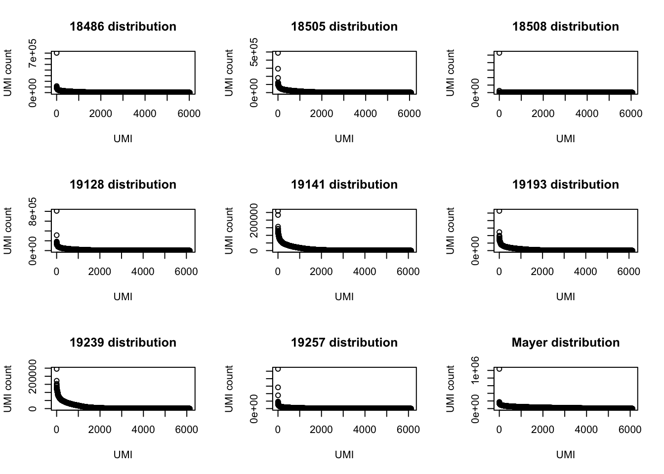 Look at the top 3 for each:
#they are sorted so the first one is the most used in that line
top_umi= c(UMI_net3_18486$umi[1], UMI_net3_18505$umi[1], UMI_net3_18508$umi[1],UMI_net3_19128$umi[1], UMI_net3_19141$umi[1], UMI_net3_19193$umi[1],UMI_net3_19239$umi[1], UMI_net3_19257$umi[1], UMI_mayer$umi[1])
sec_umi= c(UMI_net3_18486$umi[2], UMI_net3_18505$umi[2], UMI_net3_18508$umi[2],UMI_net3_19128$umi[2], UMI_net3_19141$umi[2], UMI_net3_19193$umi[2],UMI_net3_19239$umi[2], UMI_net3_19257$umi[2], UMI_mayer$umi[2])

third_umi= c(UMI_net3_18486$umi[3], UMI_net3_18505$umi[3], UMI_net3_18508$umi[3],UMI_net3_19128$umi[3], UMI_net3_19141$umi[3], UMI_net3_19193$umi[3],UMI_net3_19239$umi[3], UMI_net3_19257$umi[3], UMI_mayer$umi[3])


top3_UMI= rbind(top_umi, sec_umi, third_umi)
colnames(top3_UMI)=c(libraries, "mayer")
Seq logo plots:
require(ggseqlogo)Loading required package: ggseqlogolibrary("cowplot")Warning: package 'cowplot' was built under R version 3.4.3
Attaching package: 'cowplot'The following object is masked from 'package:ggplot2':
ggsavecs1 = make_col_scheme(chars=c('A', 'T', 'C', 'G', 'N'), groups=c('A', 'T', 'C', 'G', 'N'), cols=c('red', 'blue', 'green', 'yellow', 'pink'))gg_18486=ggseqlogo(UMI_net3_18486$umi, col_scheme=cs1)
gg_18505=ggseqlogo(UMI_net3_18505$umi, col_scheme=cs1)
gg_18508=ggseqlogo(UMI_net3_18508$umi, col_scheme=cs1)
gg_19128=ggseqlogo(UMI_net3_19128$umi, col_scheme=cs1)
gg_19141=ggseqlogo(UMI_net3_19141$umi, col_scheme=cs1)
gg_19193=ggseqlogo(UMI_net3_19193$umi, col_scheme=cs1)
gg_19239=ggseqlogo(UMI_net3_19239$umi, col_scheme=cs1)
gg_19257=ggseqlogo(UMI_net3_19257$umi, col_scheme=cs1)
gg_mayer=ggseqlogo(UMI_mayer$umi, col_scheme=cs1)plot_grid(gg_18486, gg_18505, gg_18508, gg_19128, gg_19141, gg_19193, gg_19239, gg_19257, gg_mayer, ncol=3, labels = c(libraries, "mayer"))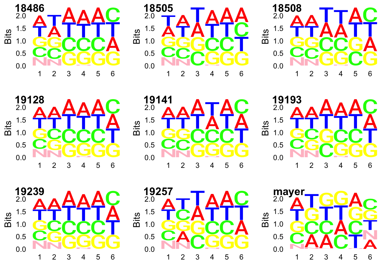
I will now use the same code on the deduplicated files so we can see if there is a descrepency is usage, this will help me know if pileup occured for one umi.
samtools view YG-SP-NET3-18486-2018-1-8_S3_L008_R1_001-sort.dedup.bam  | tr "_" "\t" | cut -f 2 | sort | uniq -c > ../../output/UMI_Net3_18486_dedupstat.txt

samtools view YG-SP-NET3-18505-2018-1-8_S1_L008_R1_001-sort.dedup.bam  | tr "_" "\t" | cut -f 2 | sort | uniq -c > ../../output/UMI_18505_dedupstat.txt

samtools view YG-SP-NET3-18508-2018-1-8_S2_L008_R1_001-sort.dedup.bam | tr "_" "\t" | cut -f 2 | sort | uniq -c > ../../output/UMI_Net3_18508_dedupstat.txt

samtools view YG-SP-NET3-19128-2018-1-8_S8_L008_R1_001-sort.dedup.bam | tr "_" "\t" | cut -f 2 | sort | uniq -c > ../../output/UMI_Net3_19128_dedupstat.txt


samtools view YG-SP-NET3-19141-2018-1-8_S5_L008_R1_001-sort.dedup.bam  | tr "_" "\t" | cut -f 2 | sort | uniq -c > ../../output/UMI_Net3_19141_dedupstat.txt


samtools view YG-SP-NET3-19193-2018-1-8_S6_L008_R1_001-sort.dedup.bam | tr "_" "\t" | cut -f 2 | sort | uniq -c > ../../output/UMI_Net3_19193_dedupstat.txt

samtools view YG-SP-NET3-19239-2018-1-8_S4_L008_R1_001-sort.dedup.bam  | tr "_" "\t" | cut -f 2 | sort | uniq -c > ../../output/UMI_Net3_19239_dedupstat.txt

samtools view YG-SP-NET3-19257-2018-1-8_S7_L008_R1_001-sort.dedup.bam | tr "_" "\t" | cut -f 2 | sort | uniq -c > ../../output/UMI_Net3_19257_dedupstat.txt
UMI_net3_18486_dedup= prepare_UMI_data("../data/UMI_Net3_18486_dedupstat.txt")
UMI_net3_18505_dedup= prepare_UMI_data("../data/UMI_Net3_18505_dedupstat.txt")
UMI_net3_18508_dedup= prepare_UMI_data("../data/UMI_Net3_18508_dedupstat.txt")
UMI_net3_19128_dedup= prepare_UMI_data("../data/UMI_Net3_19128_dedupstat.txt")
UMI_net3_19141_dedup= prepare_UMI_data("../data/UMI_Net3_19141_dedupstat.txt")
UMI_net3_19193_dedup= prepare_UMI_data("../data/UMI_Net3_19193_dedupstat.txt")
UMI_net3_19239_dedup= prepare_UMI_data("../data/UMI_Net3_19239_dedupstat.txt")
UMI_net3_19257_dedup= prepare_UMI_data("../data/UMI_Net3_19257_dedupstat.txt")
gg_18486_dedup=ggseqlogo(UMI_net3_18486_dedup$umi, col_scheme=cs1)
gg_18505_dedup=ggseqlogo(UMI_net3_18505_dedup$umi, col_scheme=cs1)
gg_18508_dedup=ggseqlogo(UMI_net3_18508_dedup$umi, col_scheme=cs1)
gg_19128_dedup=ggseqlogo(UMI_net3_19128_dedup$umi, col_scheme=cs1)
gg_19141_dedup=ggseqlogo(UMI_net3_19141_dedup$umi, col_scheme=cs1)
gg_19193_dedup=ggseqlogo(UMI_net3_19193_dedup$umi, col_scheme=cs1)
gg_19239_dedup=ggseqlogo(UMI_net3_19239_dedup$umi, col_scheme=cs1)
gg_19257_dedup=ggseqlogo(UMI_net3_19257_dedup$umi, col_scheme=cs1)
plot_grid(gg_18486_dedup, gg_18505_dedup, gg_18508_dedup, gg_19128_dedup, gg_19141_dedup, gg_19193_dedup, gg_19239_dedup, gg_19257_dedup, ncol=3, labels = c(libraries))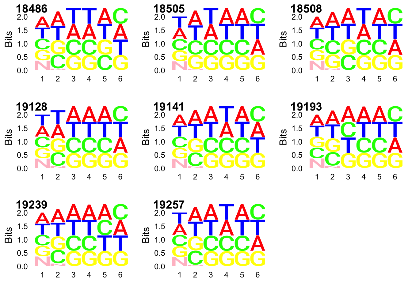 Distributions:
par(mfrow = c(3,3))
plot(UMI_net3_18486_dedup$number, ylab="UMI count", xlab="UMI", main="18486 dedup distribution")
plot(UMI_net3_18505_dedup$number, ylab="UMI count", xlab="UMI", main="18505 dedup distribution")
plot(UMI_net3_18508_dedup$number, ylab="UMI count", xlab="UMI", main="18508 dedup distribution")
plot(UMI_net3_19128_dedup$number, ylab="UMI count", xlab="UMI", main="19128 dedup distribution")
plot(UMI_net3_19141_dedup$number, ylab="UMI count", xlab="UMI", main="19141 dedup distribution")
plot(UMI_net3_19193_dedup$number, ylab="UMI count", xlab="UMI", main="19193 dedup distribution")
plot(UMI_net3_19239_dedup$number, ylab="UMI count", xlab="UMI", main="19239 dedup distribution")
plot(UMI_net3_19257_dedup$number, ylab="UMI count", xlab="UMI", main="19257 dedup distribution")
I need to merge files so I can analyze if there are differences. The problem is they are not the same size. I need a way to merge them and for the missing UMIs in the smaller file to become 0.
right_join(a, b, by = “x1”)
UMI_net3_18486_all=left_join(UMI_net3_18486, UMI_net3_18486_dedup, by="umi")
UMI_net3_18486_all[is.na(UMI_net3_18486_all)] <- 0
#column with the difference
UMI_net3_18486_all = mutate(UMI_net3_18486_all, diff= number.x- number.y)
UMI_net3_18486_all = mutate(UMI_net3_18486_all, per_diff= diff/(number.x+number.y))


summary(UMI_net3_18486_all$per_diff)
Min. 1st Qu. Median Mean 3rd Qu. Max.
0.0000 0.8935 0.9155 0.9066 0.9345 1.0000 Look at the distribution of this:
plot(UMI_net3_18486_all$per_diff)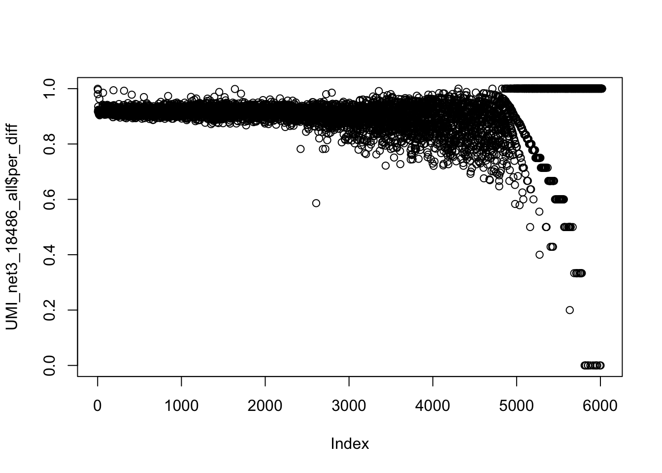 Expectation for number of times we see 1 UMI in map to the genome:
14018943/4^6 [1] 3422.594
sum(UMI_net3_18486_all$number.y >= 2000)[1] 79which(UMI_net3_18486_all$number.y ==max(UMI_net3_18486_all$number.y))[1] 3UMI analsis by position:
- Subset the sort_bam file and dedup bam file by chr 2
samtools view YG-SP-NET3-18486-2018-1-8_S3_L008_R1_001-sort.dedup.bam 2 -b > YG-SP-NET3-18486-2018-1-8_S3_L008_R1_001-sort.dedup.chr2.bam

samtools view YG-SP-NET3-18486-2018-1-8_S3_L008_R1_001-sort.bam 2 -b > YG-SP-NET3-18486-2018-1-8_S3_L008_R1_001-sort.chr2.bam- run genomecoverage -d (per base genome coverage)
chr2_coverage_18486.sh
#!/bin/bash


#SBATCH --job-name=coverage
#SBATCH --time=8:00:00
#SBATCH --partition=gilad
#SBATCH --mem=16G
#SBATCH --tasks-per-node=4
#SBATCH --mail-type=END
#SBATCH --output=coverage_sbatch.out
#SBATCH --error=coverage_sbatch.err

module load Anaconda3

source activate net-seq

bedtools genomecov -ibam /project2/gilad/briana/Net-seq/Net-seq3/data/dedup/YG-SP-NET3-18486-2018-1-8_S3_L008_R1_001-sort.dedup.chr2.bam -d > /project2/gilad/briana/Net-seq/Net-seq3/output/chr2_cov/dedup_18486_chr2.txt


bedtools genomecov -ibam  /project2/gilad/briana/Net-seq/Net-seq3/data/sort/YG-SP-NET3-18486-2018-1-8_S3_L008_R1_001-sort.chr2.bam -d > /project2/gilad/briana/Net-seq/Net-seq3/output/chr2_cov/sort_18486_chr2.txt
- plot sort coverage by dedup coverage.
Files I made are dedup_18486_chr2.txt and sort_18486_chr2.txt.
import pandas as pd
import matplotlib.pyplot as plt
dedup_18486_chr2= pd.read_csv("/project2/gilad/briana/Net-seq/Net-seq3/output/chr2_cov/dedup_18486_chr2.txt", sep="\t")
sort_18486_chr2=pd.read_csv("/project2/gilad/briana/Net-seq/Net-seq3/output/chr2_cov/sort_18486_chr2.txt", sep="\t")
2 options:
* plot pyplot from pandas dateframe
- use awk if statement to get rid of the lines where both are 0.
cut -f 3 dedup_18486_chr2.txt > count_dedup.txt
paste -d'\t' sort_18486_chr2.txt count_dedup.txt > sort_dedup_chr2_18486.txt
Now I need to get rid of the lines that are both 0:
awk '{if($3!=0 || $4!=0) print($1 "\t" $2 "\t" $3 "\t" $4)}' sort_dedup_chr2_18486.txt > sort_dedup_chr2_no0_18486.txtchr2_no0_18486=read.csv("../data/sort_dedup_chr2_no0_18486.txt", header = FALSE, sep="\t")
colnames(chr2_no0_18486)= c("chr", "pos", "sort", "dedup")
plot(chr2_no0_18486$sort ~ chr2_no0_18486$dedup, ylab = "reads", xlab="molecules", main="Reads vs molecules by position chr2")
summary(chr2_no0_18486$sort==0) Mode FALSE
logical 1356189 summary(chr2_no0_18486$dedup ==0) Mode FALSE TRUE
logical 1355227 962 I need to subset the super high expressed ones to see the distribution better.
chr2_no0_18486_sum=mutate (chr2_no0_18486, sum=chr2_no0_18486$sort + chr2_no0_18486$dedup)

chr2_no0_18486_sum_sort=arrange(chr2_no0_18486_sum, desc(sum))

#cut top 500 possitions


chr2_no0_18486_cut=chr2_no0_18486_sum_sort[which(chr2_no0_18486_sum_sort$sort<30000),]
 plot(chr2_no0_18486_cut$sort ~ chr2_no0_18486_cut$dedup, ylab = "reads", xlab="molecules", main="Reads vs molecules by position chr2")
abline(0,1) 
x=chr2_no0_18486$dedup/chr2_no0_18486$sort
summary(x)
Min. 1st Qu. Median Mean 3rd Qu. Max.
0.00000 0.01163 0.50000 0.58145 1.00000 1.00000 Specifically remove rows in the INSIG2 gene: 118843994-118869607
chr2_no0_18486_noinsig2= chr2_no0_18486[which(chr2_no0_18486$pos > 118869607 | chr2_no0_18486$pos < 118843994),]This gets rid of 22550 rows. Now I can plot again.
plot(chr2_no0_18486_noinsig2$sort ~ chr2_no0_18486_noinsig2$dedup, ylab = "reads", xlab="molecules", main="Reads vs molecules by position chr2")
abline(0,1) 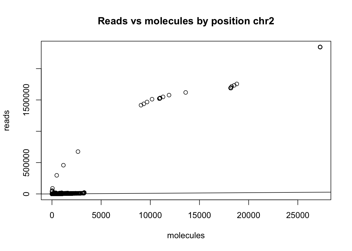 Redo this analysis but only map 3’ end of the reads.
chr2_3prime_no0_18486=read.csv("../data/sort_dedup_3prime_chr2_no0.18486.txt", header = FALSE, sep="\t")
colnames(chr2_3prime_no0_18486)= c("chr", "pos", "sort", "dedup")
plot(chr2_3prime_no0_18486$sort ~ chr2_3prime_no0_18486$dedup, ylab = "reads", xlab="molecules", main="Reads vs molecules by position chr2")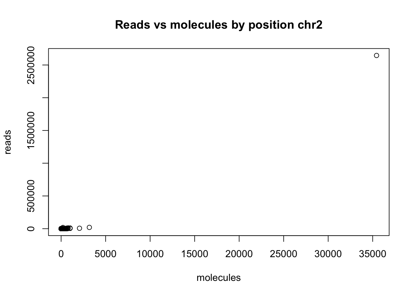 Cut that top point:
chr2_3prime_no0_18486_sum=mutate (chr2_3prime_no0_18486, sum=chr2_3prime_no0_18486$sort + chr2_3prime_no0_18486$dedup)

chr2_3prime_no0_18486_sum_sort=arrange(chr2_3prime_no0_18486_sum, desc(sum))


chr2_3prime_no0_18486_cut=chr2_3prime_no0_18486_sum_sort[which(chr2_3prime_no0_18486_sum_sort$sort<10000),]
plot(chr2_3prime_no0_18486_cut$sort ~ chr2_3prime_no0_18486_cut$dedup, ylab = "reads", xlab="molecules", main="Reads vs molecules by position chr2")
abline(0,1) 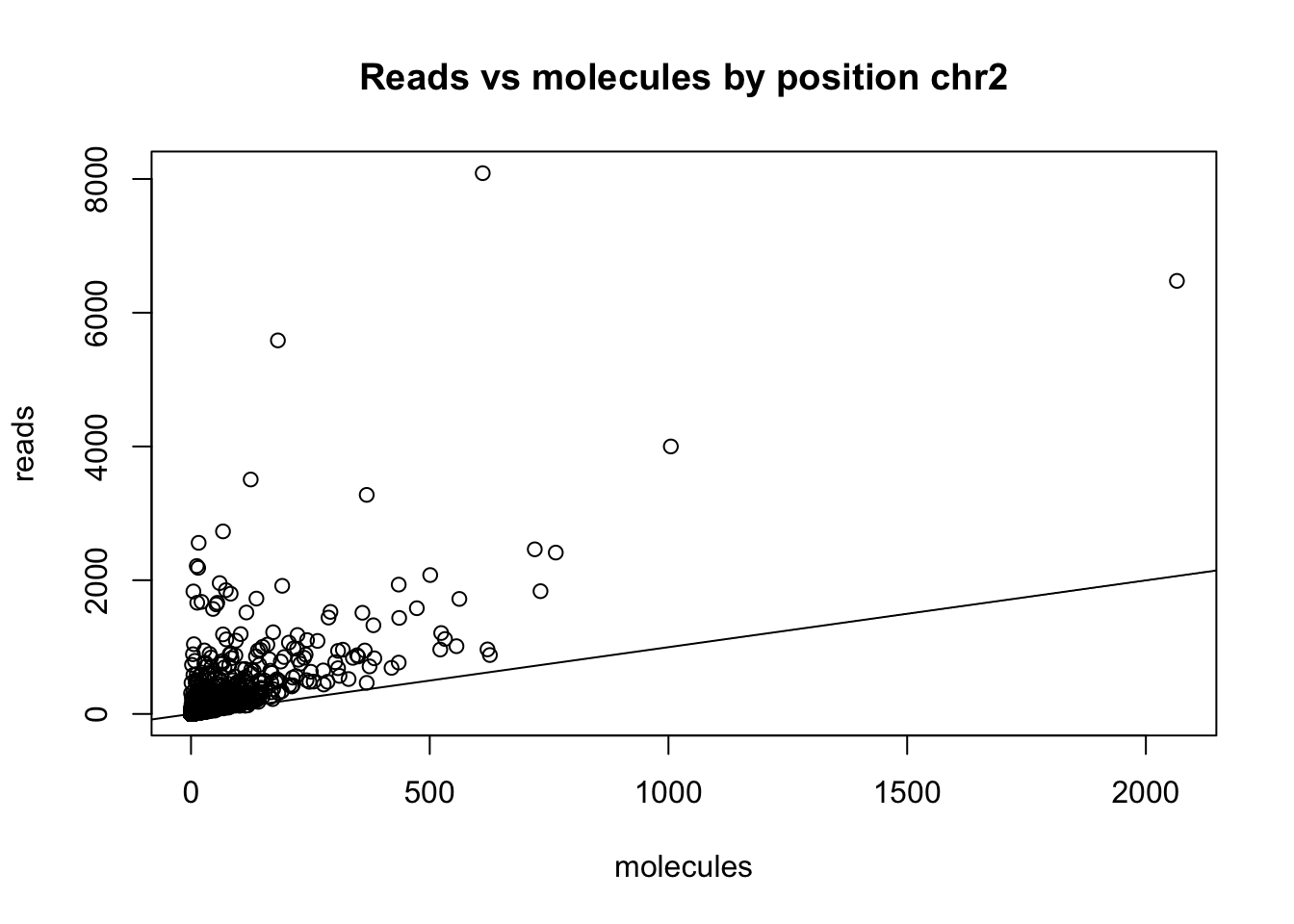
y=chr2_3prime_no0_18486$dedup/chr2_3prime_no0_18486$sort
summary(y)
Min. 1st Qu. Median Mean 3rd Qu. Max.
0.0000 0.5000 1.0000 0.8051 1.0000 1.0000 #look at top difference ones
chr2_3prime_no0_18486_sum_sort_dif= mutate(chr2_3prime_no0_18486_sum_sort, diff=chr2_3prime_no0_18486_sum_sort$sort - chr2_3prime_no0_18486_sum_sort$dedup)Coverage at splice sites
Get the 3 and 5 splice sites from the GTF file
less gencode.v19.annotation.gtf | tr "\"" "\t" | awk '$3 == "exon"'| awk "" | awk 'NR >=6 {if($7 == "+") print($1 "\t" $4 -1 "\t" $4 "\t" $10 "\t0\t" $7 ); else print($1 "\t" $5 -1 "\t" $5 "\t" $10 "\t0\t" $7 )}'  | sort -k1,1 -k2,2n > gencode.v19.5prime.gtf

less gencode.v19.annotation.gtf | tr "\"" "\t" | awk '$3 == "exon"' | awk 'NR >=6 {if($7 == "+") print($1 "\t" $5 -1 "\t" $5 "\t" $10 "\t0\t" $7 ); else print($1 "\t" $4 -1 "\t" $4 "\t" $10 "\t0\t" $7 )}'  | sort -k1,1 -k2,2n > gencode.v19.3prime.gtf
Get rid of first exon:
less gencode.v19.annotation.gtf | tr "\"" "\t" | awk '$3 == "exon"'| awk '$34 != "1;"' | awk 'NR >=6 {if($7 == "+") print($1 "\t" $4 -1 "\t" $4 "\t" $10 "\t0\t" $7 ); else print($1 "\t" $5 -1 "\t" $5 "\t" $10 "\t0\t" $7 )}'  | sort -k1,1 -k2,2n > gencode.v19.5prime.noE1.bed

less gencode.v19.annotation.gtf | tr "\"" "\t" | awk '$3 == "exon"' | awk '$34 != "1;"'| awk 'NR >=6 {if($7 == "+") print($1 "\t" $5 -1 "\t" $5 "\t" $10 "\t0\t" $7 ); else print($1 "\t" $4 -1 "\t" $4 "\t" $10 "\t0\t" $7 )}'  | sort -k1,1 -k2,2n > gencode.v19.3prime.noE1.bed
Now I need to make a TES bed file. I want 3 == gene. On the pos strand I want 4 - 300 to 4 and for the reverse strand I want 5 -300 to 5
less gencode.v19.annotation.gtf | tr "\"" "\t" | awk '$3 == "gene"'| awk 'NR >=6 {if($7 == "+") print($1 "\t" $4 - 300 "\t" $4 "\t" $10 "\t0\t" $7 ); else print($1 "\t" $5 -300 "\t" $5 "\t" $10 "\t0\t" $7 )}' | sort -k1,1 -k2,2n > gencode.v19.300TES.bedNow I want to get only the lines in the noE1 files that are not in the TES file. I will do this with bedtool intersect -v
#!/bin/bash


#SBATCH --job-name=intersect
#SBATCH --time=8:00:00
#SBATCH --partition=gilad
#SBATCH --mem=16G
#SBATCH --tasks-per-node=4
#SBATCH --mail-type=END
#SBATCH --output=intersect.sbatch.out
#SBATCH --error=intersect.sbatch.err

module load Anaconda3

source activate net-seq


bedtools intersect -v -sorted -a gencode.v19.5prime.noE1.bed -b gencode.v19.300TES.bed > gencode.v19.5prime.noE1noTES.bed


bedtools intersect -v -sorted -a gencode.v19.3prime.noE1.bed -b gencode.v19.300TES.bed > gencode.v19.3prime.noE1noTES.bed
No I will change the 5prime and 3prime deep tools scripts to use these files.
#!/bin/bash


#SBATCH --job-name=deeptools_3_netseq
#SBATCH --time=8:00:00
#SBATCH --partition=broadwl
#SBATCH --mem=30G
#SBATCH --mail-type=END
#SBATCH --output=deeptool_3_sbatch.out
#SBATCH --error=deeptools_3_sbatch.err

module load Anaconda3

source activate net-seq

#the bw file has already been created

computeMatrix reference-point -S /project2/gilad/briana/Net-seq/Net-seq3/output/deeptools/net-seq-18486.bw -R /project2/gilad/briana/Net-seq/Net-seq3/gencode.v19.3prime.gtf -b 500 -a 500 -out /project2/gilad/briana/Net-seq/Net-seq3/output/deeptools/net-seq-3prime-18486.gz

plotHeatmap --sortRegions descend --refPointLabel "3' boundary" -m /project2/gilad/briana/Net-seq/Net-seq3/output/deeptools/net-seq-3prime-18486.gz  -out /project2/gilad/briana/Net-seq/Net-seq3/output/deeptools/net-seq-3prime-18486.png
#!/bin/bash
#SBATCH --job-name=deeptools_5_netseq
#SBATCH --time=8:00:00
#SBATCH --partition=broadwl
#SBATCH --mem=30G
#SBATCH --mail-type=END
#SBATCH --output=deeptool_5_sbatch.out
#SBATCH --error=deeptools_5_sbatch.err
module load Anaconda3
source activate net-seq
#the bw file has already been created
computeMatrix reference-point -S /project2/gilad/briana/Net-seq/Net-seq3/output/deeptools/net-seq-18486.bw -R /project2/gilad/briana/Net-seq/Net-seq3/gencode.v19.3prime.gtf -b 500 -a 500 -out /project2/gilad/briana/Net-seq/Net-seq3/output/deeptools/net-seq-5prime-18486.gz
plotHeatmap --sortRegions descend --refPointLabel "5 boundary" -m /project2/gilad/briana/Net-seq/Net-seq3/output/deeptools/net-seq-5prime-18486.gz -out /project2/gilad/briana/Net-seq/Net-seq3/output/deeptools/net-seq-5prime-18486.pngNow I will seperate the genes bed file into pos and neg genes. This will seperate the genes on each strand but not strand.
I need to separate the bw files by strand as well. I do this in teh bamCoverage command with –filterRNAstrand froward and –filterRNAstrand reverse
I can the look at the difference in strand in pos then in neg genes.
Try star alligner:
#!/bin/bash

#SBATCH --job-name=star_align_net3
#SBATCH --time=8:00:00
#SBATCH --partition=broadwl
#SBATCH --mem=50G
#SBATCH --tasks-per-node=4
#SBATCH --output=star_sbatch.out
#SBATCH --error=star_sbatch.err
#SBATCH --mail-type=END


module load Anaconda3
source activate net-seq

STAR --runThreadN 4 --genomeDir /scratch/midway2/brimittleman/star_genome/ --readFilesIn /project2/gilad/briana/Net-seq/Net-seq3/data/fastq_extr/YG-SP-NET3-18486-2018-1-8_S3_L008_R1_001_extracted.fastq  --outFilterMultimapNmax 1 --outSAMtype BAM SortedByCoordinate --outStd BAM_SortedByCoordinate > /project2/gilad/briana/Net-seq/Net-seq3/data/star/star_net3-18486.bam
Output:
* Uniquely mapped reads % | 11.46%
* Average mapped length | 37.17
* % of reads unmapped: too short | 69.27%
* % of reads mapped to too many loci | 19.01%
I will run the same code with 19141.
Output:
* Uniquely mapped reads % | 14.65%
* Average mapped length | 37.90
* % of reads unmapped: too short | 63.46%
* % of reads mapped to too many loci | 21.21%
Correlations with rna seq for the same line
/project2/gilad/yangili/LCLs/bams/RNAseqGeuvadis_STAR_18486.final.bam
#!/bin/bash

#SBATCH --job-name=RNA_count_cov
#SBATCH --output=RNA_count_cov_sbatch.out
#SBATCH --error=RNA_count_cov_sbatch.err
#SBATCH --time=8:00:00
#SBATCH --partition=bigmem2
#SBATCH --mem=60G
#SBATCH --mail-type=END

module load Anaconda3

source activate net-seq


bedtools coverage -counts -sorted -a /project2/gilad/briana/Net-seq/Net-seq3/gencode.v19.annotation.sort.bed -b /project2/gilad/yangili/LCLs/bams/RNAseqGeuvadis_STAR_18486.final.bam > /project2/gilad/briana/Net-seq/Net-seq3/data/gencode_cov/RNAseqGeuvadis_STAR_18486.coverage.bed
Correlation between this and 18486,
rna_seq_cov= read.csv("../data/RNAseqGeuvadis_STAR_18486.coverage.bed", stringsAsFactors = FALSE, sep="\t", header=FALSE)
dim(net_cov_full)
[1] 99900 14dim(rna_seq_cov)[1] 99900 13plot(log(rna_seq_cov$V13)~ log(net_cov_full$`18486`))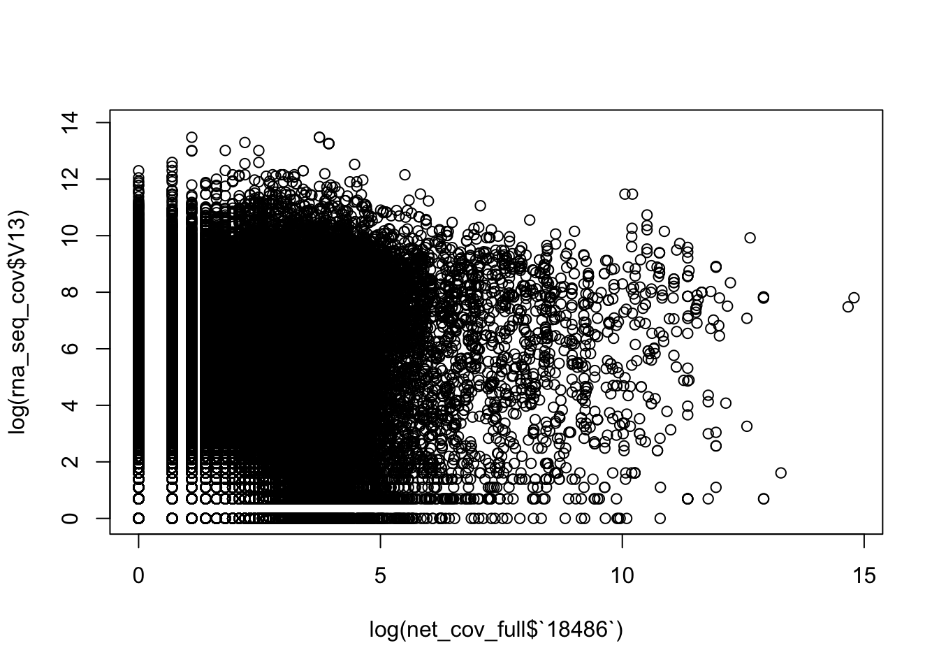
plot(rna_seq_cov$V13~ net_cov_full$`18486`)
both_18486=as.data.frame(cbind(rna_seq_cov$V13, net_cov_full$`18486`))
colnames(both_18486)=c("RNA", "Net")
cor(both_18486$RNA, both_18486$Net)
[1] -0.0003325867Need to subset this:
- extreme outliers in Net-seq
- both =0
both_18486_no0= both_18486[both_18486$Net<=30000,]
both_18486_no0 %>%
   ggplot(., aes(log(RNA), log(Net))) +
         geom_point(na.rm = TRUE, size =0.1) +
         geom_density2d(na.rm = TRUE, size = 1, colour = 'red') +
         ylab('log(RNA gene Count)') +
         xlab('Log(Net-seq gene Count)') +
        ggtitle("Counts per gene in RNAseq bs Netseq 18486")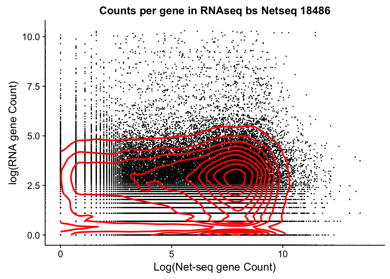
Quality of dedup mapped
/project2/gilad/briana/Net-seq/Net-seq3/data/dedup/YG-SP-NET3-18486-2018-1-8_S3_L008_R1_001-sort.dedup.bam
qual_dedup_18486=read.csv("../data/dedup_18486_mapqual.txt")
summary(qual_dedup_18486)
X13
Min. : 6.00
1st Qu.:13.00
Median :13.00
Mean :19.37
3rd Qu.:20.00
Max. :40.00 hist(qual_dedup_18486$X13)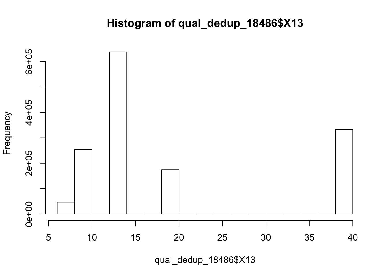
t.test(mq_18486$V1, qual_dedup_18486$X13)
    Welch Two Sample t-test

data:  mq_18486$V1 and qual_dedup_18486$X13
t = -188.18, df = 1709600, p-value < 2.2e-16
alternative hypothesis: true difference in means is not equal to 0
95 percent confidence interval:
 -1.920881 -1.881281
sample estimates:
mean of x mean of y
 17.46468  19.36576
Session information
sessionInfo()R version 3.4.2 (2017-09-28)
Platform: x86_64-apple-darwin15.6.0 (64-bit)
Running under: macOS Sierra 10.12.6
Matrix products: default
BLAS: /Library/Frameworks/R.framework/Versions/3.4/Resources/lib/libRblas.0.dylib
LAPACK: /Library/Frameworks/R.framework/Versions/3.4/Resources/lib/libRlapack.dylib
locale:
[1] en_US.UTF-8/en_US.UTF-8/en_US.UTF-8/C/en_US.UTF-8/en_US.UTF-8
attached base packages:
[1] stats graphics grDevices utils datasets methods base
other attached packages:
[1] cowplot_0.9.2 ggseqlogo_0.1 bindrcpp_0.2 dplyr_0.7.4
[5] tidyr_0.7.2 ggplot2_2.2.1 reshape2_1.4.3
loaded via a namespace (and not attached):
[1] Rcpp_0.12.15 pillar_1.1.0 compiler_3.4.2 git2r_0.21.0
[5] plyr_1.8.4 bindr_0.1 tools_3.4.2 digest_0.6.14
[9] jsonlite_1.5 evaluate_0.10.1 tibble_1.4.2 gtable_0.2.0
[13] pkgconfig_2.0.1 rlang_0.1.6 yaml_2.1.16 stringr_1.2.0
[17] knitr_1.18 rprojroot_1.3-2 grid_3.4.2 tidyselect_0.2.3
[21] reticulate_1.4 glue_1.2.0 R6_2.2.2 rmarkdown_1.8.5
[25] purrr_0.2.4 magrittr_1.5 MASS_7.3-48 backports_1.1.2
[29] scales_0.5.0 htmltools_0.3.6 assertthat_0.2.0 colorspace_1.3-2
[33] labeling_0.3 stringi_1.1.6 lazyeval_0.2.1 munsell_0.4.3 This R Markdown site was created with workflowr