Last updated: 2018-04-09

Code version: 9c9ad94

I will use this analysis to answer the question: Do eQTLs also equally affect antisense transcriptions? This will take advantage of strand specificity of the net-seq data and the phenominon of convergent and divergent transcription around TSS.

Workflow:

*Download eqtls

*Rank eqtls based on coverage in tss region, this may include seeing if the eqtl genes are in the filtered gene set from the strand specificity analysis

*Look at some of the top snps

-separate individuals by genome
-look at them in IGV
-box plots seperated by genotype, forward and reverse transcription

Load libraries

library(workflowr)

Loading required package: rmarkdown

This is workflowr version 0.7.0
Run ?workflowr for help getting started

library(tidyr)
library(dplyr)


Attaching package: 'dplyr'

The following objects are masked from 'package:stats':

    filter, lag

The following objects are masked from 'package:base':

    intersect, setdiff, setequal, union

library(reshape2)

Warning: package 'reshape2' was built under R version 3.4.3


Attaching package: 'reshape2'

The following object is masked from 'package:tidyr':

    smiths

library(ggplot2)
library(cowplot)

Warning: package 'cowplot' was built under R version 3.4.3


Attaching package: 'cowplot'

The following object is masked from 'package:ggplot2':

    ggsave

Gene overlaps

Download eqtls and YRI genotypes from http://eqtl.uchicago.edu/jointLCL/ to /project2/gilad/briana/Net-seq-pilot/data/eqtl

wget  http://eqtl.uchicago.edu/jointLCL/output_RNAseqGeuvadis_PC14.txt
wget http://eqtl.uchicago.edu/jointLCL/genotypesYRI.gen.txt.gz

Make a list of the genes that have an eqtl with the effect size (so i can order which to look at) :

awk '{print $2}' eqtl_RNAseqGeuvadis.txt > eqtl_genes
awk '{print $1 "\t" $2 "\t" $6}' eqtl_RNAseqGeuvadis.txt > eqtl_genes_effectsize.txt

The filtered genes are in /project2/gilad/briana/genome_anotation_data/gencode.v19.annotation.distfilteredgenes.bed

Pull both of these into R so I can filter the genes by if they have an eqtl.

eqtl_gene= read.table("../data/eqtl_genes_effectsize.txt", stringsAsFactors = FALSE, header=TRUE)
filter_genes= read.table("../data/gencode.v19.annotation.distfilteredgenes.bed", stringsAsFactors = FALSE)
colnames(filter_genes)=c("chr", "start", "end", "gene", "score", "strand")

Use the filter dplyr functions to filter the eqtl genes by genes that are covered in our list of filtered genes.

eqtl_gene_filter=eqtl_gene %>% semi_join(filter_genes, by="gene") %>% arrange(desc(beta))

eqtl_pergene= eqtl_gene_filter %>% group_by(gene) %>% tally()

This shows that 3985 genes in the filter_genes file have at least one eqtl. The eqtl_gene_filter file has all the eqtl genes sorted in descending order by the beta value. Now I need to back filter the bed file to only include the genes in the eqtl genes. This will allow me to get coverage for each of these.

filter_genes_byeqtl= filter_genes %>% semi_join(eqtl_pergene, by="gene")

#write.table(filter_genes_byeqtl, "../data/gencode.v19.annotation.eqtlfilter.bed",col.names = TRUE, row.names = FALSE, quote = FALSE, sep="\t")

This file is now in /project2/gilad/briana/genome_anotation_data/gencode.v19.annotation.eqtlfilter.bed

Coverage for TSS

I need to modify gencode.v19.annotation.eqtlfilter.bed to include the TSS of each of these genes. I am looking at the first 500 basepairs of each gene.

awk '{if($6 == "+") print($1 "\t" $2 -500  "\t" $2 + 500  "\t" $4 "\t" $5 "\t" $6 ); else print($1 "\t" $3 - 500 "\t" $3 +500  "\t" $4 "\t" $5 "\t" $6 )}' gencode.v19.annotation.eqtlfilter.bed  > gencode.v19.annotation.eqtlfilter_TSS.bed

Bam to bed and sort each bedfile with sort -k1,1 -k2,2n

#!/bin/bash
#SBATCH --mail-type=END

module load Anaconda3
source activate net-seq

bamToBed -i YG-SP-NET3-18508_combined_Netpilot-sort.bam | sort -k1,1 -k2,2n > ../sorted_bed/YG-SP-NET3-18508_combined_Netpilot-bedsort.bed

bamToBed -i YG-SP-NET3-19128_combined_Netpilot-sort.bam | sort -k1,1 -k2,2n > ../sorted_bed/YG-SP-NET3-19128_combined_Netpilot-bedsort.bed

bamToBed -i YG-SP-NET3-19141_combined_Netpilot-sort.bam | sort -k1,1 -k2,2n > ../sorted_bed/YG-SP-NET3-19141_combined_Netpilot-bedsort.bed

bamToBed -i YG-SP-NET3-19193_combined_Netpilot-sort.bam | sort -k1,1 -k2,2n > ../sorted_bed/YG-SP-NET3-19193_combined_Netpilot-bedsort.bed

bamToBed -i YG-SP-NET3-19239_combined_Netpilot-sort.bam | sort -k1,1 -k2,2n > ../sorted_bed/YG-SP-NET3-19239_combined_Netpilot-bedsort.bed

bamToBed -i YG-SP-NET3-19257_combined_Netpilot-sort.bam | sort -k1,1 -k2,2n > ../sorted_bed/YG-SP-NET3-19257_combined_Netpilot-bedsort.bed

Now I can write a script that counts the coverage for these TSS in a strand specific manner. Remeber that netseq is flipped strand so same strand should be the -S and opp strand is -s. This script is in the code directory and is called eqtl_stranded.sh.

#!/bin/bash

#SBATCH --job-name=eqtl_strand
#SBATCH --time=8:00:00
#SBATCH --output=eqtlstrand.out
#SBATCH --error=eqtlstrand.err
#SBATCH --partition=broadwl
#SBATCH --mem=40G
#SBATCH --mail-type=END

module load Anaconda3
source activate net-seq  

sample=$1
describer=$(echo ${sample} | sed -e 's/.*\YG-SP-//' | sed -e "s/_combined_Netpilot-bedsort.bed$//")


bedtools coverage -counts -S -a /project2/gilad/briana/genome_anotation_data/gencode.v19.annotation.eqtlfilter_TSS.bed -b $1 > /project2/gilad/briana/Net-seq-pilot/output/eqtl_strand_spec/${describer}_same_eqtstrandedlTSS.txt

bedtools coverage -counts -s -a /project2/gilad/briana/genome_anotation_data/gencode.v19.annotation.eqtlfilter_TSS.bed -b $1 > /project2/gilad/briana/Net-seq-pilot/output/eqtl_strand_spec/${describer}_opp_eqtstrandedlTSS.txt

Create a wrapper to run this on all files: wrap_eqtl_strand.sh

#!/bin/bash

#SBATCH --job-name=w_eqtl_strand
#SBATCH --time=8:00:00
#SBATCH --output=weqtlstrand.out
#SBATCH --error=weqtlstrand.err
#SBATCH --partition=broadwl
#SBATCH --mem=8G
#SBATCH --mail-type=END


for i in $(ls /project2/gilad/briana/Net-seq-pilot/data/sorted_bed/); do
            sbatch eqtl_stranded.sh /project2/gilad/briana/Net-seq-pilot/data/sorted_bed/$i 
        done

need to give more memory to 508, 128, 141, 193, 239

Pull in all files and join them the same strand ones on the first four columns

same_18486= read.table(file = "../data/eqtl_strand_spec/NET3-18486_same_eqtstrandedlTSS.txt", header =F, col.names=c("chr", "start", "end", "gene", "score", "strand", "s_18486"), stringsAsFactors = F)
same_18505= read.table(file = "../data/eqtl_strand_spec/NET3-18505_same_eqtstrandedlTSS.txt", header =F, col.names=c("chr", "start", "end", "gene", "score", "strand", "s_18505"),stringsAsFactors = F)
same_18508= read.table(file = "../data/eqtl_strand_spec/NET3-18508_same_eqtstrandedlTSS.txt", header =F, col.names=c("chr", "start", "end", "gene", "score", "strand", "s_18508"),stringsAsFactors = F)
same_19128= read.table(file = "../data/eqtl_strand_spec/NET3-19128_same_eqtstrandedlTSS.txt", header =F, col.names=c("chr", "start", "end", "gene", "score", "strand", "s_19128"),stringsAsFactors = F)
same_19141= read.table(file = "../data/eqtl_strand_spec/NET3-19141_same_eqtstrandedlTSS.txt", header =F, col.names=c("chr", "start", "end", "gene", "score", "strand", "s_19141"),stringsAsFactors = F)
same_19193= read.table(file = "../data/eqtl_strand_spec/NET3-19193_same_eqtstrandedlTSS.txt", header =F, col.names=c("chr", "start", "end", "gene", "score", "strand", "s_19193"),stringsAsFactors = F)
same_19239= read.table(file = "../data/eqtl_strand_spec/NET3-19239_same_eqtstrandedlTSS.txt", header =F, col.names=c("chr", "start", "end", "gene", "score", "strand", "s_19239"),stringsAsFactors = F)
same_19257= read.table(file = "../data/eqtl_strand_spec/NET3-19257_same_eqtstrandedlTSS.txt", header =F, col.names=c("chr", "start", "end", "gene", "score", "strand", "s_19257"),stringsAsFactors = F)

Normalize by the number of mapped reads:

mapreads_18486=65189389
mapreads_18505=52507749
mapreads_18508=105741388
mapreads_19128=115999510
mapreads_19141=98490544
mapreads_19193=113382430
mapreads_19239=113178636
mapreads_19257=74321615

same_18486 = same_18486 %>% mutate(same_18486n =(s_18486+1)/mapreads_18486)
same_18505= same_18505 %>% mutate(same_18505n = (s_18505 +1)/mapreads_18505)
same_18508=same_18508 %>% mutate(same_18508n =(s_18508 +1)/mapreads_18508)
same_19128=same_19128 %>% mutate(same_19128n =(s_19128 +1)/mapreads_19128)
same_19141=same_19141 %>% mutate(same_19141n = (s_19141 +1)/mapreads_19141)
same_19193 = same_19193%>% mutate(same_19193n =(s_19193 +1)/mapreads_19193)
same_19239 =same_19239%>% mutate(same_19239n =(s_19239 +1)/mapreads_19239)
same_19257 =same_19257%>% mutate(same_19257n =(s_19257 +1)/mapreads_19257)

Same strand:

all_same_strand=cbind(same_18486[,1:6],same_18486$same_18486n, same_18505$same_18505n, same_18508$same_18508n, same_19128$same_19128n,same_19141$same_19141n, same_19193$same_19193n, same_19239$same_19239n, same_19257$same_19257n)
colnames(all_same_strand)=c("chr", "start", "end", "gene", "score", "strand", "same_18486", "same_18505", "same_18508", "same_19128", "same_19141", "same_19193", "same_19239", "same_19257")


all_same_strand_long=melt(all_same_strand, variable.name = "library",  value.name = "same_count",
                     id.vars = c("chr", "start", "end", "gene", "score", "strand"))

plot coverage dist:

ggplot(all_same_strand_long, aes(x=library, y=(same_count))) + geom_violin()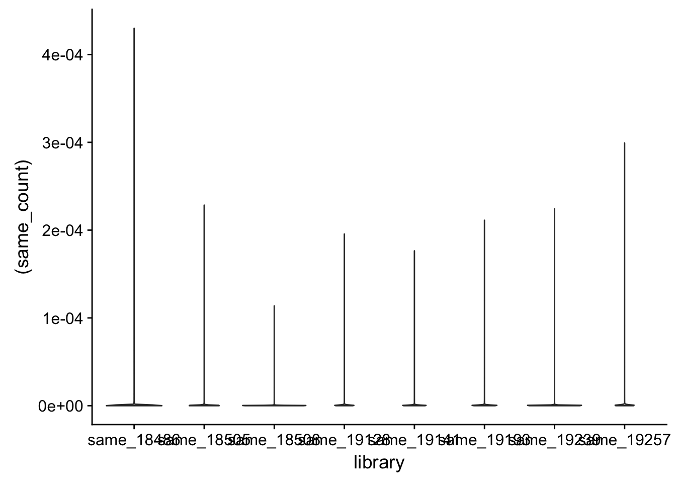

Opp strand:

opp_18486= read.table(file = "../data/eqtl_strand_spec/NET3-18486_opp_eqtstrandedlTSS.txt", header =F, col.names=c("chr", "start", "end", "gene", "score", "strand", "o_18486"),stringsAsFactors = F)
opp_18505= read.table(file = "../data/eqtl_strand_spec/NET3-18505_opp_eqtstrandedlTSS.txt", header =F, col.names=c("chr", "start", "end", "gene", "score", "strand", "o_18505"),stringsAsFactors = F)
opp_18508= read.table(file = "../data/eqtl_strand_spec/NET3-18508_opp_eqtstrandedlTSS.txt", header =F, col.names=c("chr", "start", "end", "gene", "score", "strand", "o_18508"),stringsAsFactors = F)
opp_19128= read.table(file = "../data/eqtl_strand_spec/NET3-19128_opp_eqtstrandedlTSS.txt", header =F, col.names=c("chr", "start", "end", "gene", "score", "strand", "o_19128"),stringsAsFactors = F)
opp_19141= read.table(file = "../data/eqtl_strand_spec/NET3-19141_opp_eqtstrandedlTSS.txt", header =F, col.names=c("chr", "start", "end", "gene", "score", "strand", "o_19141"),stringsAsFactors = F)
opp_19193= read.table(file = "../data/eqtl_strand_spec/NET3-19193_opp_eqtstrandedlTSS.txt", header =F, col.names=c("chr", "start", "end", "gene", "score", "strand", "o_19193"),stringsAsFactors = F)
opp_19239= read.table(file = "../data/eqtl_strand_spec/NET3-19239_opp_eqtstrandedlTSS.txt", header =F, col.names=c("chr", "start", "end", "gene", "score", "strand", "o_19239"),stringsAsFactors = F)
opp_19257= read.table(file = "../data/eqtl_strand_spec/NET3-19257_opp_eqtstrandedlTSS.txt", header =F, col.names=c("chr", "start", "end", "gene", "score", "strand", "o_19257"),stringsAsFactors = F)

opp_18486 = opp_18486 %>% mutate(opp_18486n = (o_18486 +1) /mapreads_18486)
opp_18505= opp_18505 %>% mutate(opp_18505n =(o_18505 + 1)/mapreads_18505)
opp_18508=opp_18508 %>% mutate(opp_18508n =(o_18508 + 1)/mapreads_18508)
opp_19128=opp_19128 %>% mutate(opp_19128n =(o_19128 +1)/mapreads_19128)
opp_19141=opp_19141 %>% mutate(opp_19141n =(o_19141 +1)/mapreads_19141)
opp_19193 = opp_19193%>% mutate(opp_19193n =(o_19193+1)/mapreads_19193)
opp_19239 =opp_19239%>% mutate(opp_19239n =(o_19239+1)/mapreads_19239)
opp_19257 =opp_19257%>% mutate(opp_19257n =(o_19257+1)/mapreads_19257)

all_opp_strand=cbind(opp_18486[,1:7], opp_18505$opp_18505n, opp_18508$opp_18508n, opp_19128$opp_19128n,opp_19141$opp_19141n, opp_19193$opp_19193n, opp_19239$opp_19239n, opp_19257$opp_19257n)
colnames(all_opp_strand)=c("chr", "start", "end", "gene", "score", "strand", "opp_18486", "opp_18505", "opp_18508", "opp_19128", "opp_19141", "opp_19193", "opp_19239", "opp_19257")

all_opp_strand_long=melt(all_opp_strand, variable.name = "library",  value.name = "opp_count",
                     id.vars = c("chr", "start", "end", "gene", "score", "strand"))
ggplot(all_opp_strand_long, aes(x=library, y=log10(opp_count + .25))) + geom_violin()

Combine these to do it together colored by strand.

colnames(all_same_strand)= c("chr", "start", "end", "gene", "score", "strand", "l_18486", "l_18505", "l_18508", "l_19128", "l_19141", "l_19193", "l_19239", "l_19257")
all_same_strand_new= all_same_strand %>% mutate(which_strand="same")


colnames(all_opp_strand)= c("chr", "start", "end", "gene", "score", "strand", "l_18486", "l_18505", "l_18508", "l_19128", "l_19141", "l_19193", "l_19239", "l_19257")
all_opp_strand_new=all_opp_strand %>% mutate(which_strand="opp")

all_coverage= rbind(all_same_strand_new, all_opp_strand_new)

Make this long:

all_strand_long=melt(all_coverage, variable.name = "library", value.name = "count",
                     id.vars = c("chr", "start", "end", "gene", "score", "strand", "which_strand"))


ggplot(all_strand_long, aes(x=library, y=log10( count+ .25), fill=which_strand)) + geom_violin() + ggtitle("TSS coverage by strand by libary")

Calculate the %same:

perc_18486=all_same_strand$l_18486/(all_same_strand$l_18486 + all_opp_strand$l_18486)
perc_18505=all_same_strand$l_18505/(all_same_strand$l_18505 + all_opp_strand$l_18505)
perc_18508=all_same_strand$l_18508/(all_same_strand$l_18508 + all_opp_strand$l_18508)
perc_19128=all_same_strand$l_19128/(all_same_strand$l_19128 + all_opp_strand$l_19128)
perc_19141=all_same_strand$l_19141/(all_same_strand$l_19141 + all_opp_strand$l_19141)
perc_19193=all_same_strand$l_19193/(all_same_strand$l_19193 + all_opp_strand$l_19193)
perc_19239=all_same_strand$l_19239/(all_same_strand$l_19239 + all_opp_strand$l_19239)
perc_19257=all_same_strand$l_19257/(all_same_strand$l_19257 + all_opp_strand$l_19257)

Create a table with these:

perc_all= cbind(all_same_strand[,1:6],perc_18486,perc_18505,perc_18508,perc_19128,perc_19141,perc_19193, perc_19239,perc_19257)

Make this tidy to remove NA and to make box plots

perc_all_long=melt(perc_all, variable.name = "library",  value.name = "perc_same",
                     id.vars = c("chr", "start", "end", "gene", "score", "strand"), na.rm = TRUE)

Make a side by side box plot:

ggplot(perc_all_long, aes(x=library, y=perc_same)) + geom_violin() + ggtitle("Distribution of the precent of reads mapping to the same strand")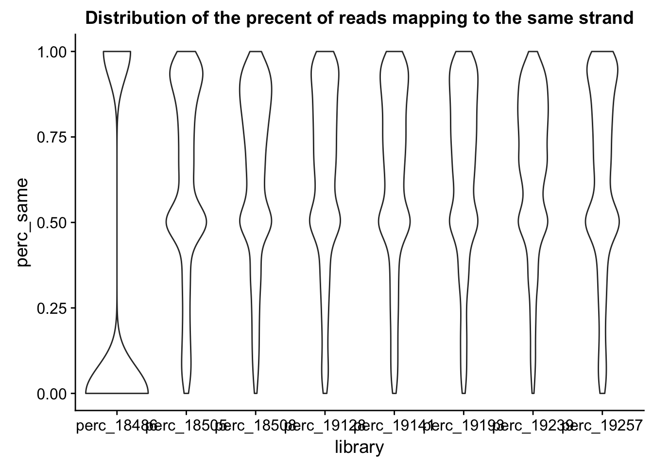

This is good. Expectation is the samples have similar distributions of the

Look at eqtls

I need to select the genotypes by the individuals i have and the eqtl snps.

geno= read.table("../data/eqtl_strand_spec/genotypesYRI.gen.txt")
colnames(geno)= c("CHROM",  "POS",  "ID",   "REF",  "ALT",  "QUAL", "FILTER",   "INFO", "FORMAT",   "18486",    "18489",    "18498",    "18499",    "18501",    "18502",    "18504",    "18505",    "18507",    "18508",    "18510",    "18511",    "18516",    "18517",    "18519",    "18520",    "18522",    "18523",    "18853",    "18856",    "18858",    "18861",    "18870",    '18871',    "18907",    "18909",    "18912",    "18916",    "19093",    "19098",    "19099",    '19102',    "19108",    "19114",    "19116",    "19119",    "19129",    "19131",    '19137',    "19138",    "19141",    "19143",    "19144",    "19147",    "19152",    "19153",    "19159",    "19160",    "19171",    "19172",    "19190",    "19200",    "19201",    "19204",    "19207",    "19209",    "19210",    "19225",    "19257",    "19175",    "19176",    "19203",    "18855",    "19095",    "19096",    "18867",    "18868",    "18924",    "18923",    "18488",    "19122",    "19121",    "19247",    "19248",    "18933",    "18934",    "19118",    '19117',    '19149',    "19150",    "18487",    "19235",    "19236",    "19226",    "19189",    "18910",    "18917",    "19113",    "19214",    "19213",    "19182",    "19181",    "19179",    "19178",    "19146",    "19107",    "19185",    "19184",    "19256",    "19197",    "19198",    "18873",    "18874",    "19238",    "19239",    "19222",    "19223",    "18862",    "18852",    "19140",    "19127",    "19128",    "19193",    "19192",    "19130",    "19206",    "18913",    '18859',    "19101")

filter by my ind.:

geno_netpilot= geno %>% select("CHROM", "POS",  "ID",   "REF",  "ALT",  "QUAL", "FILTER",   "INFO", "FORMAT", "18486", "18505", "18508", "19128", "19141", "19193", "19239", "19257")

Write out this filitered data:

write.table(geno_netpilot, "../data/eqtl_strand_spec/genotypesYRI.gen.netpilot.txt", quote=FALSE,strcol.names = c("CHROM",  "POS",  "ID",   "REF",  "ALT",  "QUAL", "FILTER",   "INFO", "FORMAT", "18486", "18505", "18508", "19128", "19141", "19193", "19239", "19257"))

Pull this in for analysis:

geno_netpilot= read.table( "../data/eqtl_strand_spec/genotypesYRI.gen.netpilot.txt", header=TRUE, stringsAsFactors = FALSE)

The next step will be to filter this further by the eqtl snps, to do this i will have to process the eqtl snp ids by seperating the chr and the rs ids. I will then be able to filter join with dplyr.

eqtl_gene_filter_rs= eqtl_gene_filter %>% separate(snps,c("CHROM", "ID"))

eqtl_gene_filter_rs$ID=sub("^", "rs", eqtl_gene_filter_rs$ID)

Use semi joing by the CHROM and ID columns. I want to filter the genotypes so that is the x.

geno_netpilot_eqtl=geno_netpilot %>% semi_join(eqtl_gene_filter_rs, by=c("ID"))
geno_netpilot_eqtl_round= geno_netpilot_eqtl %>% mutate_if(is.numeric, round)

Create a file with the full count for each gene at its TSS by adding the strand counts:

all_18486=all_same_strand$l_18486 + all_opp_strand$l_18486
all_18505=all_same_strand$l_18505+ all_opp_strand$l_18505
all_18508=all_same_strand$l_18508 + all_opp_strand$l_18508
all_19128=all_same_strand$l_19128 + all_opp_strand$l_19128
all_19141=all_same_strand$l_19141 + all_opp_strand$l_19141
all_19193=all_same_strand$l_19193 + all_opp_strand$l_19193
all_19239=all_same_strand$l_19239+ all_opp_strand$l_19239
all_19257=all_same_strand$l_19257+ all_opp_strand$l_19257


all_exp_both= cbind(all_same_strand[,1:6],all_18486,all_18505,all_18508, all_19128,all_19141,all_19193, all_19239, all_19257)

Next step is to create the function that plots the gene coverage by genotype when you give it a qtl snp:

by_geno_exp=function(rsID){
  geno_rs=geno_netpilot_eqtl_round %>% filter(geno_netpilot_eqtl_round$ID==rsID) %>% select(10:17)
  gene_rs= eqtl_gene_filter_rs  %>% filter(ID==rsID) %>% select(gene) %>% top_n(1) %>% as.character()
  beta= eqtl_gene_filter_rs  %>% filter(ID==rsID) %>% select(beta) %>% top_n(1) %>% as.character()
  exp_gene= all_exp_both %>% filter(gene==gene_rs) %>% select(7:14)
  colnames(exp_gene)= colnames(geno_rs)
  x=rbind(geno_rs,exp_gene) %>% t
  x=as.data.frame(x)
  x$V1=as.factor(x$V1)
  plot=ggplot(x, aes(y=log10(V2), x=V1)) + geom_boxplot() + geom_jitter(col="red") + ggtitle(paste(rsID,":eqtl beta=",round(as.numeric(beta),2))) + xlab("Genotype") + ylab("log 10 normalized count")
  return(plot)
}

Sort the eqtls by effect size and run my function on top 10:

top_10_effect=eqtl_gene_filter_rs %>% arrange(desc(beta))  %>% semi_join(geno_netpilot_eqtl_round, by="ID") %>%  semi_join(all_exp_both, by="gene") %>%  top_n(20) %>% select(ID)

Selecting by beta

print(top_10_effect)

            ID
1  rs142833498
2     rs583662
3     rs581956
4     rs579627
5     rs579713
6     rs579450
7     rs577760
8     rs580388
9     rs576932
10    rs573205
11    rs572878
12    rs574927
13    rs575083
14    rs575159
15  rs74234805
16  rs11883894
17    rs259304
18    rs260747
19   rs7268500
20    rs260142
21    rs260182

rs142833498_plot=by_geno_exp("rs142833498")

Selecting by gene

Selecting by beta

rs583662_plot=by_geno_exp("rs583662")

Selecting by gene
Selecting by beta

rs579627_plot=by_geno_exp("rs579627")

Selecting by gene
Selecting by beta

rs74234805_plot=by_geno_exp("rs74234805")

Selecting by gene
Selecting by beta

rs259304_plot=by_geno_exp("rs259304")

Selecting by gene
Selecting by beta

rs260142plot=by_geno_exp("rs260142")

Selecting by gene
Selecting by beta

plot_grid(rs142833498_plot,rs583662_plot,rs579627_plot,rs74234805_plot,rs259304_plot,rs260142plot)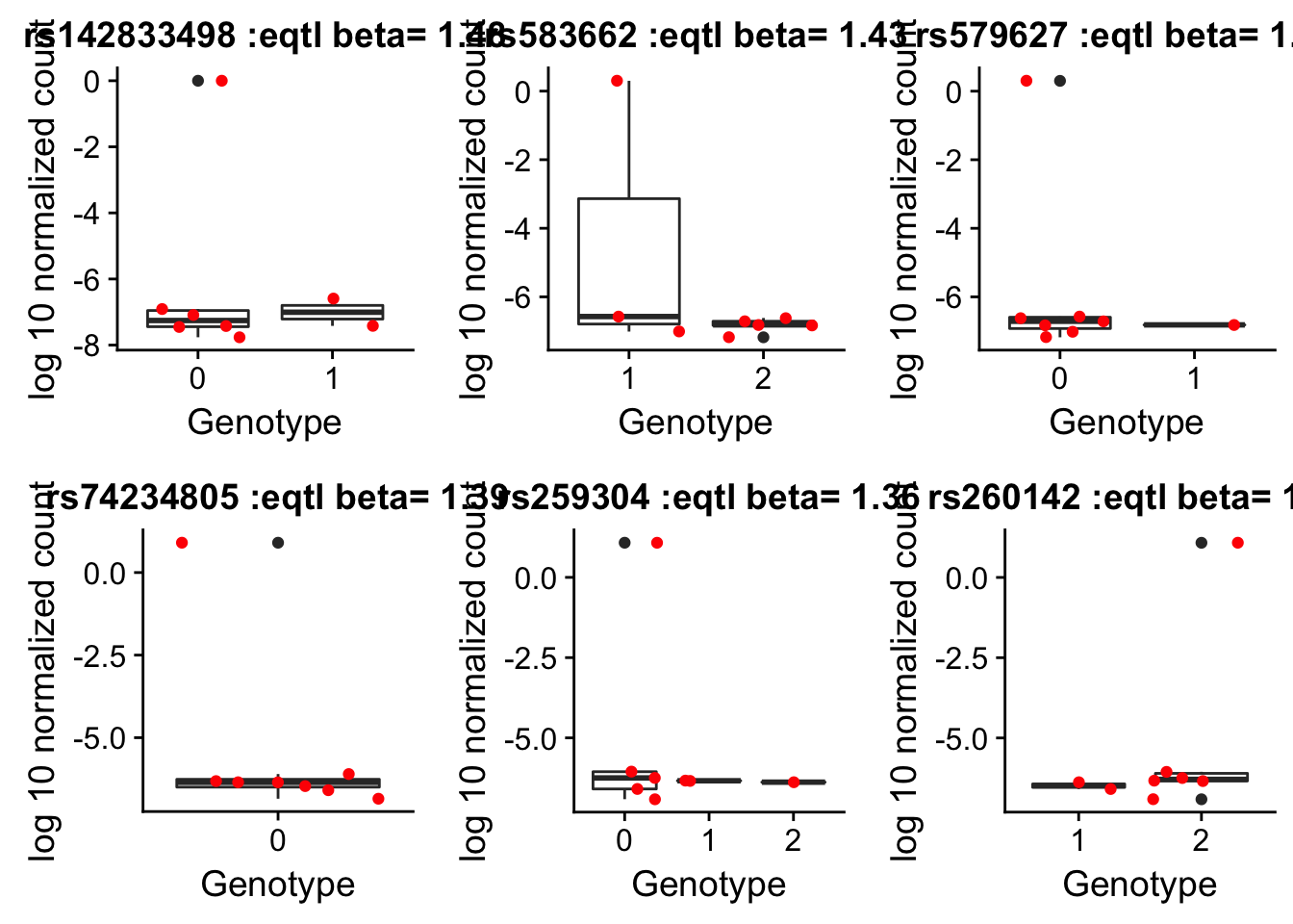

There are 16362 eqtls that we have genotype and expression information for.

Whole gene body analysis

I need to do this analysis but using the number of reads mapping to each gene rather than just around the TSS. For this I need to make a coverage file with gencode.v19.annotation.eqtlfilter.bed

I will make this script eqtlcov_fullgene.sh

#!/bin/bash

#SBATCH --job-name=eqtl_full
#SBATCH --time=8:00:00
#SBATCH --output=eqtlfull.out
#SBATCH --error=eqtlfull.err
#SBATCH --partition=bigmem2
#SBATCH --mem=80G
#SBATCH --mail-type=END

module load Anaconda3
source activate net-seq  

sample=$1
describer=$(echo ${sample} | sed -e 's/.*\YG-SP-//' | sed -e "s/_combined_Netpilot-bedsort.bed$//")

bedtools coverage -counts -sorted -S -a /project2/gilad/briana/genome_anotation_data/gencode.v19.annotation.eqtlfilter.bed -b $1 > /project2/gilad/briana/Net-seq-pilot/output/eqtl_fullgene/${describer}_same_eqtstranded_fullgene.txt

bedtools coverage -counts -sorted -s -a /project2/gilad/briana/genome_anotation_data/gencode.v19.annotation.eqtlfilter.bed -b $1 > /project2/gilad/briana/Net-seq-pilot/output/eqtl_fullgene/${describer}_opp_eqtstranded_fullgene.txt

I will also create a wrapper to run this on all of the lines:

#!/bin/bash

#SBATCH --job-name=w_eqtl_full
#SBATCH --time=8:00:00
#SBATCH --output=weqtlfull.out
#SBATCH --error=weqtlfull.err
#SBATCH --partition=broadwl
#SBATCH --mem=8G
#SBATCH --mail-type=END


for i in $(ls /project2/gilad/briana/Net-seq-pilot/data/sorted_bed/); do
            sbatch eqtlcov_fullgene.sh /project2/gilad/briana/Net-seq-pilot/data/sorted_bed/$i  
        done

Pull in the data and combine the strand to get the full gene count regardless of strand.

s_18486_gene=read.table("../data/eqtl_fullgene/NET3-18486_same_eqtstranded_fullgene.txt", header =F, col.names=c("chr", "start", "end", "gene", "score", "strand", "s_18486"), stringsAsFactors = F)

s_18505_gene=read.table("../data/eqtl_fullgene/NET3-18505_same_eqtstranded_fullgene.txt", header =F, col.names=c("chr", "start", "end", "gene", "score", "strand", "s_18505"), stringsAsFactors = F)

s_18508_gene=read.table("../data/eqtl_fullgene/NET3-18508_same_eqtstranded_fullgene.txt", header =F, col.names=c("chr", "start", "end", "gene", "score", "strand", "s_18508"), stringsAsFactors = F)

s_19128_gene=read.table("../data/eqtl_fullgene/NET3-19128_same_eqtstranded_fullgene.txt", header =F, col.names=c("chr", "start", "end", "gene", "score", "strand", "s_19128"), stringsAsFactors = F)

s_19141_gene=read.table("../data/eqtl_fullgene/NET3-19141_same_eqtstranded_fullgene.txt", header =F, col.names=c("chr", "start", "end", "gene", "score", "strand", "s_19141"), stringsAsFactors = F)

s_19193_gene=read.table("../data/eqtl_fullgene/NET3-19193_same_eqtstranded_fullgene.txt", header =F, col.names=c("chr", "start", "end", "gene", "score", "strand", "s_19193"), stringsAsFactors = F)

s_19239_gene=read.table("../data/eqtl_fullgene/NET3-19239_same_eqtstranded_fullgene.txt", header =F, col.names=c("chr", "start", "end", "gene", "score", "strand", "s_19239"), stringsAsFactors = F)

s_19257_gene=read.table("../data/eqtl_fullgene/NET3-19257_same_eqtstranded_fullgene.txt", header =F, col.names=c("chr", "start", "end", "gene", "score", "strand", "s_19257"), stringsAsFactors = F)

o_18486_gene=read.table("../data/eqtl_fullgene/NET3-18486_opp_eqtstranded_fullgene.txt", header =F, col.names=c("chr", "start", "end", "gene", "score", "strand", "o_18486"), stringsAsFactors = F)

o_18505_gene=read.table("../data/eqtl_fullgene/NET3-18505_opp_eqtstranded_fullgene.txt", header =F, col.names=c("chr", "start", "end", "gene", "score", "strand", "o_18505"), stringsAsFactors = F)

o_18508_gene=read.table("../data/eqtl_fullgene/NET3-18508_opp_eqtstranded_fullgene.txt", header =F, col.names=c("chr", "start", "end", "gene", "score", "strand", "o_18508"), stringsAsFactors = F)

o_19128_gene=read.table("../data/eqtl_fullgene/NET3-19128_opp_eqtstranded_fullgene.txt", header =F, col.names=c("chr", "start", "end", "gene", "score", "strand", "o_19128"), stringsAsFactors = F)

o_19141_gene=read.table("../data/eqtl_fullgene/NET3-19141_opp_eqtstranded_fullgene.txt", header =F, col.names=c("chr", "start", "end", "gene", "score", "strand", "o_19141"), stringsAsFactors = F)

o_19193_gene=read.table("../data/eqtl_fullgene/NET3-19193_opp_eqtstranded_fullgene.txt", header =F, col.names=c("chr", "start", "end", "gene", "score", "strand", "o_19193"), stringsAsFactors = F)

o_19239_gene=read.table("../data/eqtl_fullgene/NET3-19239_opp_eqtstranded_fullgene.txt", header =F, col.names=c("chr", "start", "end", "gene", "score", "strand", "o_19239"), stringsAsFactors = F)

o_19257_gene=read.table("../data/eqtl_fullgene/NET3-19257_opp_eqtstranded_fullgene.txt", header =F, col.names=c("chr", "start", "end", "gene", "score", "strand", "o_19257"), stringsAsFactors = F)

Create a total count dataframe for each line by joining the files, adding a column with 1 + total/mapped reads.

t_18486_gene= s_18486_gene %>% left_join(o_18486_gene, by=c("chr", "start", "end", "gene", "score", "strand")) %>% mutate(tot_18486=(1+ s_18486 + o_18486)/mapreads_18486)


t_18505_gene= s_18505_gene %>% left_join(o_18505_gene, by=c("chr", "start", "end", "gene", "score", "strand")) %>% mutate(tot_18505=(1+ s_18505 + o_18505)/mapreads_18505)

t_18508_gene= s_18508_gene %>% left_join(o_18508_gene, by=c("chr", "start", "end", "gene", "score", "strand")) %>% mutate(tot_18508=(1+ s_18508 + o_18508)/mapreads_18508)

t_19128_gene= s_19128_gene %>% left_join(o_19128_gene, by=c("chr", "start", "end", "gene", "score", "strand")) %>% mutate(tot_19128=(1+ s_19128 + o_19128)/mapreads_19128)

t_19141_gene= s_19141_gene %>% left_join(o_19141_gene, by=c("chr", "start", "end", "gene", "score", "strand")) %>% mutate(tot_19141=(1+ s_19141 + o_19141)/mapreads_19141)

t_19193_gene= s_19193_gene %>% left_join(o_19193_gene, by=c("chr", "start", "end", "gene", "score", "strand")) %>% mutate(tot_19193=(1+ s_19193 + o_19193)/mapreads_19193)

t_19239_gene= s_19239_gene %>% left_join(o_19239_gene, by=c("chr", "start", "end", "gene", "score", "strand")) %>% mutate(tot_19239=(1+ s_19239 + o_19239)/mapreads_19239)


t_19257_gene= s_19257_gene %>% left_join(o_19257_gene, by=c("chr", "start", "end", "gene", "score", "strand")) %>% mutate(tot_19257=(1+ s_19257 + o_19257)/mapreads_19257)

Left join all of these by c(“chr”, “start”, “end”, “gene”, “score”, “strand”)

all_exp_gene= cbind(t_18486_gene[1:6], t_18486_gene$tot_18486, t_18505_gene$tot_18505, t_18508_gene$tot_18508, t_19128_gene$tot_19128, t_19141_gene$tot_19141, t_19193_gene$tot_19193, t_19239_gene$tot_19239, t_19257_gene$tot_19257)

Create a new function to make the graph.

by_geno_exp_gene=function(rsID){
  geno_rs=geno_netpilot_eqtl_round %>% filter(geno_netpilot_eqtl_round$ID==rsID) %>% select(10:17)
  gene_rs= eqtl_gene_filter_rs  %>% filter(ID==rsID) %>% select(gene) %>% top_n(1) %>% as.character()
  beta= eqtl_gene_filter_rs  %>% filter(ID==rsID) %>% select(beta) %>% top_n(1) %>% as.character()
  #chaned to all_exp_gene to include not just TSS 
  exp_gene= all_exp_gene %>% filter(gene==gene_rs) %>% select(7:14)
  colnames(exp_gene)= colnames(geno_rs)
  x=rbind(geno_rs,exp_gene) %>% t
  x=as.data.frame(x)
  x$V1=as.factor(x$V1)
  plot=ggplot(x, aes(y=log10(V2), x=V1)) + geom_boxplot() + geom_jitter(col="red") + ggtitle(paste(rsID,":eqtl beta=",round(as.numeric(beta),2))) + xlab("Genotype") + ylab("log 10 normalized count")
  return(plot)
}

rs142833498_plot_g=by_geno_exp_gene("rs142833498")

Selecting by gene

Selecting by beta

rs583662_plot_g=by_geno_exp_gene("rs583662")

Selecting by gene
Selecting by beta

rs579627_plot_g=by_geno_exp_gene("rs579627")

Selecting by gene
Selecting by beta

rs74234805_plot_g=by_geno_exp_gene("rs74234805")

Selecting by gene
Selecting by beta

rs259304_plot_g=by_geno_exp_gene("rs259304")

Selecting by gene
Selecting by beta

rs260142plot_g=by_geno_exp_gene("rs260142")

Selecting by gene
Selecting by beta

plot_grid(rs142833498_plot_g,rs583662_plot_g,rs579627_plot_g,rs74234805_plot_g,rs259304_plot_g,rs260142plot_g)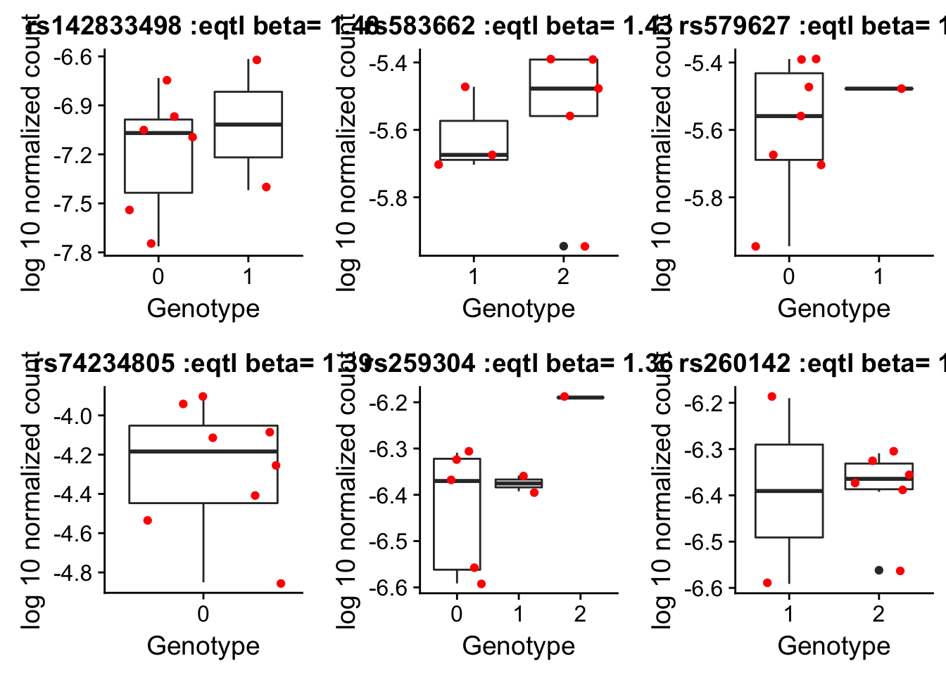

Session information

sessionInfo()

R version 3.4.2 (2017-09-28)
Platform: x86_64-apple-darwin15.6.0 (64-bit)
Running under: macOS Sierra 10.12.6

Matrix products: default
BLAS: /Library/Frameworks/R.framework/Versions/3.4/Resources/lib/libRblas.0.dylib
LAPACK: /Library/Frameworks/R.framework/Versions/3.4/Resources/lib/libRlapack.dylib

locale:
[1] en_US.UTF-8/en_US.UTF-8/en_US.UTF-8/C/en_US.UTF-8/en_US.UTF-8

attached base packages:
[1] stats     graphics  grDevices utils     datasets  methods   base     

other attached packages:
[1] bindrcpp_0.2    cowplot_0.9.2   ggplot2_2.2.1   reshape2_1.4.3 
[5] dplyr_0.7.4     tidyr_0.7.2     workflowr_0.7.0 rmarkdown_1.8.5

loaded via a namespace (and not attached):
 [1] Rcpp_0.12.15     knitr_1.18       bindr_0.1        magrittr_1.5    
 [5] tidyselect_0.2.3 munsell_0.4.3    colorspace_1.3-2 R6_2.2.2        
 [9] rlang_0.1.6      plyr_1.8.4       stringr_1.2.0    tools_3.4.2     
[13] grid_3.4.2       gtable_0.2.0     git2r_0.21.0     htmltools_0.3.6 
[17] lazyeval_0.2.1   yaml_2.1.16      rprojroot_1.3-2  digest_0.6.14   
[21] assertthat_0.2.0 tibble_1.4.2     purrr_0.2.4      glue_1.2.0      
[25] evaluate_0.10.1  labeling_0.3     stringi_1.1.6    compiler_3.4.2  
[29] pillar_1.1.0     scales_0.5.0     backports_1.1.2  pkgconfig_2.0.1

This R Markdown site was created with workflowr