Characterize orthologous peaks

Last updated: 2018-08-28

workflowr checks: (Click a bullet for more information)

✔ R Markdown file: up-to-date

Great! Since the R Markdown file has been committed to the Git repository, you know the exact version of the code that produced these results.
✔ Environment: empty

Great job! The global environment was empty. Objects defined in the global environment can affect the analysis in your R Markdown file in unknown ways. For reproduciblity it’s best to always run the code in an empty environment.
✔ Seed: set.seed(20180801)

The command set.seed(20180801) was run prior to running the code in the R Markdown file. Setting a seed ensures that any results that rely on randomness, e.g. subsampling or permutations, are reproducible.
✔ Session information: recorded

Great job! Recording the operating system, R version, and package versions is critical for reproducibility.
✔ Repository version: bfa1099
Great! You are using Git for version control. Tracking code development and connecting the code version to the results is critical for reproducibility. The version displayed above was the version of the Git repository at the time these results were generated.

Note that you need to be careful to ensure that all relevant files for the analysis have been committed to Git prior to generating the results (you can use wflow_publish or wflow_git_commit). workflowr only checks the R Markdown file, but you know if there are other scripts or data files that it depends on. Below is the status of the Git repository when the results were generated:
```
Ignored files:
    Ignored:    .RData
    Ignored:    .Rhistory
    Ignored:    .Rproj.user/

Untracked files:
    Untracked:  com_threeprime.Rproj
    Untracked:  data/PeakPerExon/
    Untracked:  data/PeakPerGene/
    Untracked:  data/comp.pheno.data.csv
    Untracked:  data/dist_TES/
    Untracked:  data/dist_upexon/
    Untracked:  data/liftover/
    Untracked:  data/map.stats.csv
    Untracked:  data/map.stats.xlsx
    Untracked:  data/orthoPeak_quant/

Unstaged changes:
    Deleted:    comparitive_threeprime.Rproj
```
Note that any generated files, e.g. HTML, png, CSS, etc., are not included in this status report because it is ok for generated content to have uncommitted changes.

Expand here to see past versions:

File	Version	Author	Date	Message
Rmd	bfa1099	brimittleman	2018-08-28	fix format
html	f2fa4e1	brimittleman	2018-08-28	Build site.
Rmd	1ae2e49	brimittleman	2018-08-28	fix format
html	1f8f5b1	brimittleman	2018-08-28	Build site.
Rmd	8f61cee	brimittleman	2018-08-28	add plot recreating wang et al 2018
html	a237865	brimittleman	2018-08-24	Build site.
Rmd	364f330	brimittleman	2018-08-24	TES distance
html	d11c2cf	brimittleman	2018-08-22	Build site.
Rmd	3a19b07	brimittleman	2018-08-22	add hg19 dist
html	d0d4599	brimittleman	2018-08-21	Build site.

I will use this analysis for QC on the orthologous peaks called in the liftover pipeline analysis.

Distance to ortho exon

I want to make sure the distances of the orthologous peaks to the nearest exon called in Bryans ortho exon files follow a similar distribution.

The orthologus exon files are in /project2/gilad/briana/genome_anotation_data/ortho_exon and the small version have just chr start end and exon name.

The ortho peak files are in /project2/gilad/briana/comparitive_threeprime/data/ortho_peaks/

I want the closest exon upstream, i will use bedtools closest:

distUpstreamexon.sh

#!/bin/bash

#SBATCH --job-name=disUpstreamexon
#SBATCH --account=pi-yangili1
#SBATCH --time=24:00:00
#SBATCH --output=disUpstreamexon.out
#SBATCH --error=disUpstreamexon.err
#SBATCH --partition=broadwl
#SBATCH --mem=12G
#SBATCH --mail-type=END


module load Anaconda3
source activate comp_threeprime_env

bedtools closest -id -D a -a /project2/gilad/briana/comparitive_threeprime/data/ortho_peaks/chimpOrthoPeaks.sort.bed  -b /project2/gilad/briana/genome_anotation_data/ortho_exon/2017_July_ortho_chimp.small.sort.bed > /project2/gilad/briana/comparitive_threeprime/data/dist_upexon/Chimp.distUpstreamexon.txt


bedtools closest -id -D a -a /project2/gilad/briana/comparitive_threeprime/data/ortho_peaks/humanOrthoPeaks.sort.bed -b /project2/gilad/briana/genome_anotation_data/ortho_exon/2017_July_ortho_human.small.sort.bed > /project2/gilad/briana/comparitive_threeprime/data/dist_upexon/Human.distUpstreamexon.txt

Import the files and plot the distances.

library(tidyverse)

── Attaching packages ─────────────────────────────────────────────────── tidyverse 1.2.1 ──

✔ ggplot2 3.0.0     ✔ purrr   0.2.5
✔ tibble  1.4.2     ✔ dplyr   0.7.6
✔ tidyr   0.8.1     ✔ stringr 1.3.1
✔ readr   1.1.1     ✔ forcats 0.3.0

── Conflicts ────────────────────────────────────────────────────── tidyverse_conflicts() ──
✖ dplyr::filter() masks stats::filter()
✖ dplyr::lag()    masks stats::lag()

library(workflowr)

This is workflowr version 1.1.1
Run ?workflowr for help getting started

library(cowplot)


Attaching package: 'cowplot'

The following object is masked from 'package:ggplot2':

    ggsave

library(reshape2)


Attaching package: 'reshape2'

The following object is masked from 'package:tidyr':

    smiths

getwd()

[1] "/Users/bmittleman1/Documents/Gilad_lab/comparitive_threeprime/com_threeprime/analysis"

file.exists("../data/dist_upexon/Chimp.distUpstreamexon.txt")

[1] TRUE

chimp_dist=read.table("../data/dist_upexon/Chimp.distUpstreamexon.txt", col.names = c("peak_chr", "peak_start", "peak_end", "peak_name", "exon_chr", "exon_start", "exon_end", "exon_name", "dist"), stringsAsFactors = F) %>% mutate(logdis=log10(abs(dist) +1 ))

human_dist=read.table("../data/dist_upexon/Human.distUpstreamexon.txt", col.names = c("peak_chr", "peak_start", "peak_end", "peak_name", "exon_chr", "exon_start", "exon_end", "exon_name", "dist"),stringsAsFactors = F, skip=1) %>% mutate(logdis=log10(abs(dist) +1 ))

ch=ggplot(chimp_dist, aes(x=logdis)) + geom_density() + labs(x="log10 abs.value \n distance +1 ", title="Chimp distance to ortho exon")

hu=ggplot(human_dist, aes(x=logdis)) + geom_density()+ labs(x="log10 abs.value \n distance +1 ", title="Human distance to ortho exon")


plot_grid(ch, hu)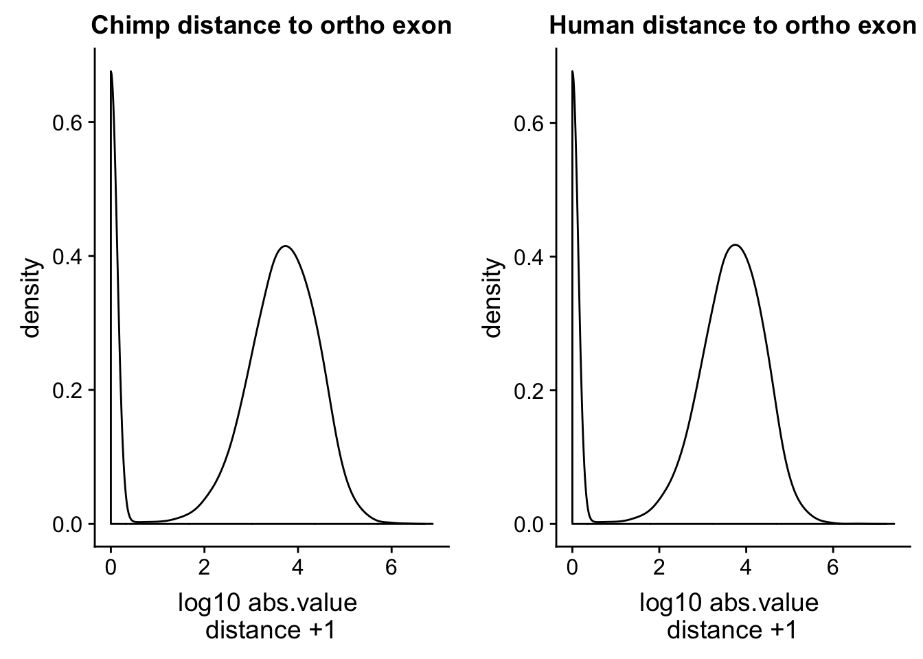

Expand here to see past versions of unnamed-chunk-4-1.png:

Version	Author	Date
d0d4599	brimittleman	2018-08-21

This is a good sanity check. The distributions are similar. I want to check this with the peaks from the human APAqtl study. I have the gencode exons and I will run bedtools cloests with this.

#!/bin/bash

#SBATCH --job-name=disUpstreamexon_hum
#SBATCH --account=pi-yangili1
#SBATCH --time=24:00:00
#SBATCH --output=disUpstreamexon_hum.out
#SBATCH --error=disUpstreamexon_hum.err
#SBATCH --partition=broadwl
#SBATCH --mem=12G
#SBATCH --mail-type=END


module load Anaconda3
source activate comp_threeprime_env

bedtools closest -id -D a -a /project2/gilad/briana/comparitive_threeprime/data/extra_anno/human_hg19_filteredPeaks.bed -b /project2/gilad/briana/comparitive_threeprime/data/extra_anno/gencode.hg19.v19.exons.bed > /project2/gilad/briana/comparitive_threeprime/data/dist_upexon/hg19.humanpeaks.distUpstreamexon.txt

update these files to remove the tab at the end.

hg19_dist=read.table("../data/dist_upexon/hg19.humanpeaks.distUpstreamexon.txt", col.names = c("peak_chr", "peak_start", "peak_end", "peak_cov","peak_strand", "peak_score", "exon_chr", "exon_start", "exon_end", "exon_name", "exon_score", "exon_strand", "dist"),stringsAsFactors = F, skip=1) %>% mutate(logdis=log10(abs(dist) +1 ))

ggplot(hg19_dist, aes(x=logdis)) + geom_density()+ labs(x="log10 abs.value \n distance +1 ", title="Hg19 peaks dist to upstream exon")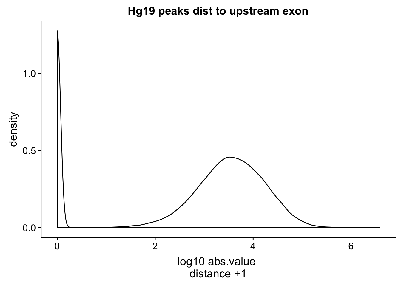

Expand here to see past versions of unnamed-chunk-6-1.png:

Version	Author	Date
d11c2cf	brimittleman	2018-08-22

How many per gene:

This is the code from the human apa qtl study. I used this to count how many peaks map to each gene. I will do this for the human and chimp here.

#!/bin/bash

#SBATCH --job-name=mapgene2peak2
#SBATCH --account=pi-yangili1
#SBATCH --time=24:00:00
#SBATCH --output=mapgene2peak2.out
#SBATCH --error=mapgene2peak2.err
#SBATCH --partition=broadwl
#SBATCH --mem=12G
#SBATCH --mail-type=END

module load Anaconda3
source activate three-prime-env


bedtools map -c 4 -o count_distinct -a /project2/gilad/briana/genome_anotation_data/gencode.v19.annotation.proteincodinggene.bed -b /project2/gilad/briana/threeprimeseq/data/clean.peaks_comb/APApeaks_combined_clean_fixed.bed > /project2/gilad/briana/threeprimeseq/data/clean.peaks_comb/APApeaks_combined_clean_countdistgenes.txt

I need to create bed files for the protein coding genes. For the human file the mRNAs are labeled with NM. The gene id is column 2, chr is column 3, strand is 4, start is 5, end is 6.

First I keep only the NM ones with:

 grep "NM" humanGene_ncbiRefSeq.txt > humanGene_ncbiRefSeq_mRNA.txt
 
 awk '{print $3 "\t" $5 "\t" $6 "\t" $2 "\t" "." "\t" $4 }' humanGene_ncbiRefSeq_mRNA.txt > humanGene_ncbiRefSeq_mRNA.bed
 
 grep "NM"  chimpGene_refGene.txt  >  chimpGene_refGene_mRNA.txt 
 
 awk '{print $3 "\t" $5 "\t" $6 "\t" $2 "\t" "." "\t" $4 }'  chimpGene_refGene_mRNA.txt >  chimpGene_refGene_mRNA.bed

#!/bin/bash

#SBATCH --job-name=PeakPerGene
#SBATCH --account=pi-yangili1
#SBATCH --time=24:00:00
#SBATCH --output=PeakPerGene.out
#SBATCH --error=PeakPerGene.err
#SBATCH --partition=broadwl
#SBATCH --mem=12G
#SBATCH --mail-type=END

module load Anaconda3
source activate comp_threeprime_env


bedtools map -c 4 -o count_distinct -a /project2/gilad/briana/genome_anotation_data/comp_genomes/gene_annos/humanGene_ncbiRefSeq_mRNA_sort.bed -b /project2/gilad/briana/comparitive_threeprime/data/ortho_peaks/humanOrthoPeaks.sort.bed > /project2/gilad/briana/comparitive_threeprime/data/PeakPerGene/humanOrthoPeakPerGene.bed



bedtools map -c 4 -o count_distinct -a /project2/gilad/briana/genome_anotation_data/comp_genomes/gene_annos/chimpGene_refGene_mRNA_sort.bed -b /project2/gilad/briana/comparitive_threeprime/data/ortho_peaks/chimpOrthoPeaks.sort.bed > /project2/gilad/briana/comparitive_threeprime/data/PeakPerGene/chimpOrthoPeakPerGene.bed

human_peakpergene= read.table("../data/PeakPerGene/humanOrthoPeakPerGene.bed", header=F, stringsAsFactors = F,col.names = c("chr", "start", "end", "gene", "score", "strand", "numPeaks")) %>% mutate(spec= "H") 

summary(human_peakpergene$numPeaks)

   Min. 1st Qu.  Median    Mean 3rd Qu.    Max. 
  0.000   0.000   0.000   3.924   3.000 206.000

chimp_peakpergene= read.table("../data/PeakPerGene/chimpOrthoPeakPerGene.bed", stringsAsFactors = F, header = F, col.names = c("chr", "start", "end", "gene", "score", "strand", "numPeaks")) %>% mutate(spec="C") 


summary(chimp_peakpergene$numPeaks)

   Min. 1st Qu.  Median    Mean 3rd Qu.    Max. 
  0.000   0.000   0.000   2.684   3.000  95.000

humanPPG=ggplot(human_peakpergene, aes(x=log10(numPeaks))) + geom_density(fill="Red") + labs(title="Peaks per Gene \n Human mRNA")
chimpPPG=ggplot(chimp_peakpergene, aes(x=log10(numPeaks))) + geom_density(fill="Blue") + labs(title="Peaks per Gene \n Chimp mRNA")
plot_grid(humanPPG, chimpPPG)

Warning: Removed 27137 rows containing non-finite values (stat_density).

Warning: Removed 1218 rows containing non-finite values (stat_density).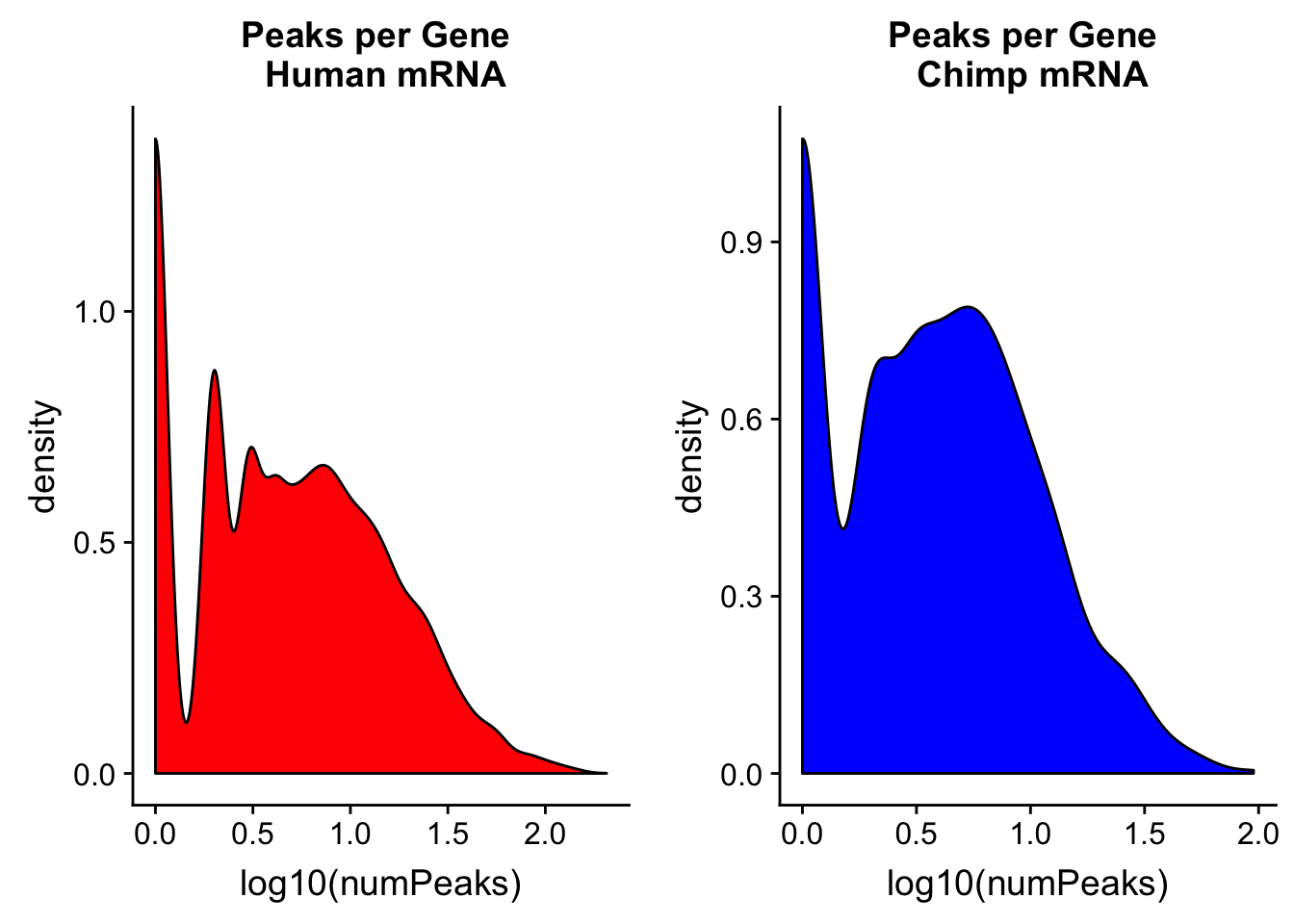

Expand here to see past versions of unnamed-chunk-11-1.png:

Version	Author	Date
a237865	brimittleman	2018-08-24

Genes with conserved PAS

I will follow a similar strategy to Wang et al. 2018 to make a plot similar to plot 1d. I want the percent of genes in both species with conserved PAS.

chimp_peakpergene= chimp_peakpergene %>% mutate(oneConservedPeak=ifelse(numPeaks==1, 1, 0 )) %>% mutate(multConservedPeak= ifelse(numPeaks > 1, 1, 0))


Cgenes1peak=sum(chimp_peakpergene$oneConservedPeak)/nrow(chimp_peakpergene)
CgenesMultpeak=sum(chimp_peakpergene$multConservedPeak)/nrow(chimp_peakpergene)
Cgenes0peak=1- CgenesMultpeak - Cgenes1peak

human_peakpergene = human_peakpergene %>% mutate(oneConservedPeak=ifelse(numPeaks==1, 1,0)) %>% mutate(multConservedPeak=ifelse(numPeaks >1,1,0))


Hgenes1peak=sum(human_peakpergene$oneConservedPeak) / nrow(human_peakpergene) 
HgenesMultpeak=sum(human_peakpergene$multConservedPeak)/ nrow(human_peakpergene)
Hgenes0peak=1- HgenesMultpeak - Hgenes1peak

I want to create a data frame with these numbers to plot it.

Hgene_peak=c(Hgenes0peak,Hgenes1peak,HgenesMultpeak)
Cgene_peak=c(Cgenes0peak, Cgenes1peak, CgenesMultpeak)
both_gene_peak=as.data.frame(rbind(Hgene_peak, Cgene_peak))
colnames(both_gene_peak)= c("ZeroConserved", "OneConserved", "MultConserved")
rownames(both_gene_peak)=c("Human", "Chimp")
both_gene_peak= both_gene_peak %>% rownames_to_column(var="Species")

both_gene_peak_melt=melt(both_gene_peak, id.vars ="Species")

#add average number of conserved peak per gene 
avgH=round(mean(human_peakpergene$numPeaks),digits = 3)
avgC=round(mean(chimp_peakpergene$numPeaks),digits = 3)

Plot this:

genepeakplot= ggplot(both_gene_peak_melt, aes(x=Species, fill=variable, y=value)) + geom_bar(stat="identity", position = "fill") + labs(y="Prop of Protein Coding Genes", title="Conserved peaks \n in protein coding genes") + scale_fill_discrete(name = "Number of \nConserved Peaks", labels=c("Zero","One", "Multiple")) + annotate("text", x=1, y=.8, label= paste("avg peaks\n per gene \n", avgH, sep=" ")) + annotate("text", x = 2, y=.8, label = paste("avg peaks\n per gene \n", avgC, sep=" "))
  
genepeakplot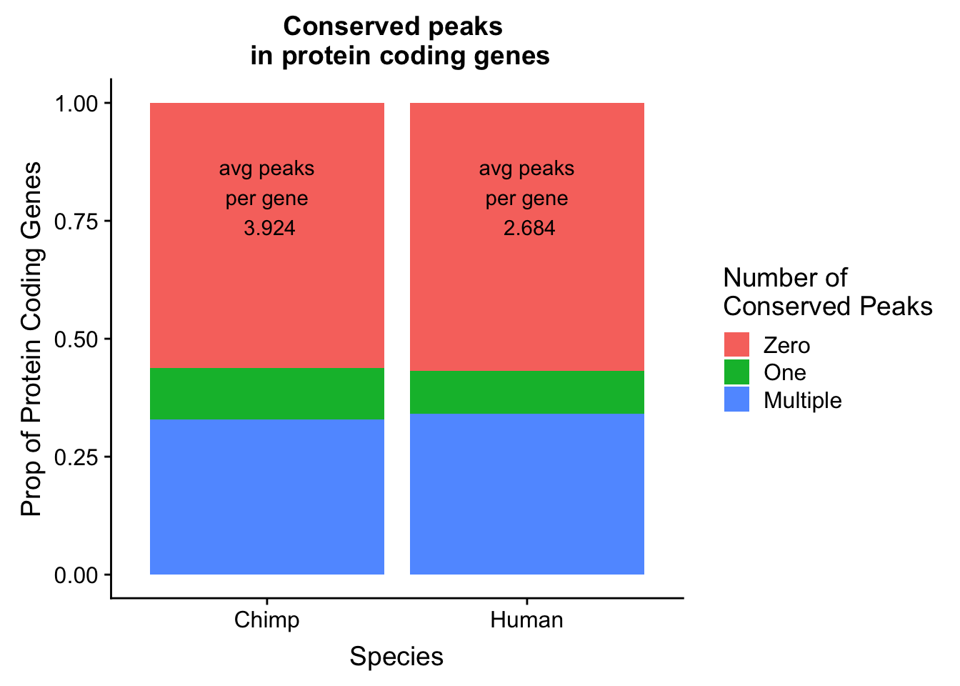

Expand here to see past versions of unnamed-chunk-14-1.png:

Version	Author	Date
1f8f5b1	brimittleman	2018-08-28
a237865	brimittleman	2018-08-24

Conserved exons

I can run similar code on the conserved exons. We expect similar distribution but most of the exons will have 0. This is the primary reason to use conserved peaks in three prime bias data.

#!/bin/bash

#SBATCH --job-name=PeakPerExon
#SBATCH --account=pi-yangili1
#SBATCH --time=24:00:00
#SBATCH --output=PeakPerExon.out
#SBATCH --error=PeakPerExon.err
#SBATCH --partition=broadwl
#SBATCH --mem=12G
#SBATCH --mail-type=END

module load Anaconda3
source activate comp_threeprime_env


bedtools map -c 4 -o count_distinct -a /project2/gilad/briana/genome_anotation_data/ortho_exon/2017_July_ortho_human.small.sort.bed -b /project2/gilad/briana/comparitive_threeprime/data/ortho_peaks/humanOrthoPeaks.sort.bed > /project2/gilad/briana/comparitive_threeprime/data/PeakPerGene/humanOrthoPeakPerExon.bed



bedtools map -c 4 -o count_distinct -a /project2/gilad/briana/genome_anotation_data/ortho_exon/2017_July_ortho_chimp.small.sort.bed -b /project2/gilad/briana/comparitive_threeprime/data/ortho_peaks/chimpOrthoPeaks.sort.bed > /project2/gilad/briana/comparitive_threeprime/data/PeakPerGene/chimpOrthoPeakPerExon.bed

file.exists("../data/PeakPerExon/humanOrthoPeakPerExon.bed")

[1] TRUE

human_peakperexon= read.table("../data/PeakPerExon/humanOrthoPeakPerExon.bed", header=F, stringsAsFactors = F,col.names = c("chr", "start", "end", "exon", "numPeaks")) %>% mutate(spec= "H") 

summary(human_peakperexon$numPeaks)

    Min.  1st Qu.   Median     Mean  3rd Qu.     Max. 
 0.00000  0.00000  0.00000  0.06772  0.00000 13.00000

chimp_peakperexon= read.table("../data/PeakPerExon/chimpOrthoPeakPerExon.bed", stringsAsFactors = F, header = F, col.names = c("chr", "start", "end", "exon", "numPeaks")) %>% mutate(spec="C") 


summary(chimp_peakperexon$numPeaks)

    Min.  1st Qu.   Median     Mean  3rd Qu.     Max. 
 0.00000  0.00000  0.00000  0.06766  0.00000 13.00000

humanPPE=ggplot(human_peakperexon, aes(x=numPeaks)) + geom_density(fill="Red") + labs(title="Peaks per Exon \n Human")
chimpPPE=ggplot(chimp_peakperexon, aes(x=numPeaks)) + geom_density(fill="Blue") + labs(title="Peaks per Exon \n Chimp ")
plot_grid(humanPPE, chimpPPE)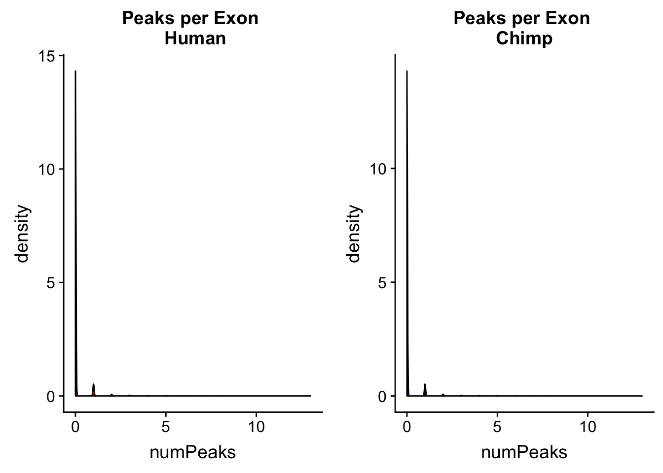

Expand here to see past versions of unnamed-chunk-17-1.png:

Version	Author	Date
1f8f5b1	brimittleman	2018-08-28

Most of the exons have 0 peaks. This is expected. I want to look at how many 0s, 1s ect we have in each data set.

human_exoncounts=human_peakperexon %>% count(numPeaks)

chimp_exoncounts=chimp_peakperexon %>% count(numPeaks)


both_exon=human_exoncounts %>% left_join(chimp_exoncounts, by="numPeaks")

colnames(both_exon)=c("PeakNum", "Human", "Chimp")


both_exon_melt=melt(both_exon, measure.vars =c("Human", "Chimp"))


ggplot(both_exon_melt, aes(x=PeakNum, y=value, col=variable)) + geom_point( size=3) + facet_grid(~variable) + labs(y="Exons", title="Number of peaks per conserved exons")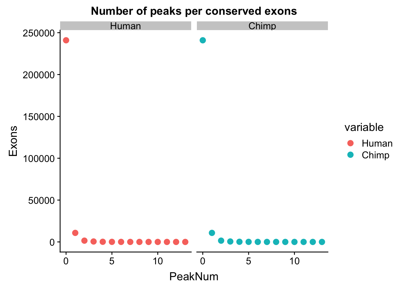

Expand here to see past versions of unnamed-chunk-18-1.png:

Version	Author	Date
1f8f5b1	brimittleman	2018-08-28
a237865	brimittleman	2018-08-24

Distance to TES

I want to look at the peaks distance to annotated gene TES in each species. I can make TES files by using the gene file. I need to take into account the strand. For the pos strand I use the end but for the neg strand I need to use the start. The easiest way to do this is in python. The scripts are called human_tes.py and chimp_tes.py

#!/bin/bash

#SBATCH --job-name=disTES
#SBATCH --account=pi-yangili1
#SBATCH --time=24:00:00
#SBATCH --output=disTES.out
#SBATCH --error=disTES.err
#SBATCH --partition=broadwl
#SBATCH --mem=12G
#SBATCH --mail-type=END


module load Anaconda3
source activate comp_threeprime_env


bedtools closest -id -D a -a /project2/gilad/briana/comparitive_threeprime/data/ortho_peaks/humanOrthoPeaks.sort.bed -b /project2/gilad/briana/genome_anotation_data/comp_genomes/gene_annos/humanGene_ncbiRefSeq_TES_sort.bed > /project2/gilad/briana/comparitive_threeprime/data/dist_TES/Human.distTES.txt

bedtools closest -id -D a -a /project2/gilad/briana/comparitive_threeprime/data/ortho_peaks/chimpOrthoPeaks.sort.bed  -b /project2/gilad/briana/genome_anotation_data/comp_genomes/gene_annos/chimpGene_refGene_TES_sort.bed > /project2/gilad/briana/comparitive_threeprime/data/dist_TES/Chimp.distTES.txt

tes_names=c("peakchr", "peakstart", "peakend", "peakname", "genechr", "geneTES_S", "geneTES_E", "gene", "score", "strand", "dist")
human_TESdis=read.table("../data/dist_TES/Human.distTES.txt", stringsAsFactors = F,col.names = tes_names ) %>% mutate(logdis=log10(abs(dist)+1))

chimp_TESdist= read.table("../data/dist_TES/Chimp.distTES.txt", stringsAsFactors = F, col.names = tes_names) %>% mutate(logdis=log10(abs(dist) + 1))

chTES=ggplot(chimp_TESdist, aes(x=logdis)) + geom_density(fill="blue") + labs(title="Distance to TES \n Chimp",x="Log10 distance + 1")

huTES=ggplot(human_TESdis, aes(x=logdis)) + geom_density(fill="red") + labs(title="Distance to TES \n Human",x="Log10 distance + 1")


plot_grid(huTES, chTES)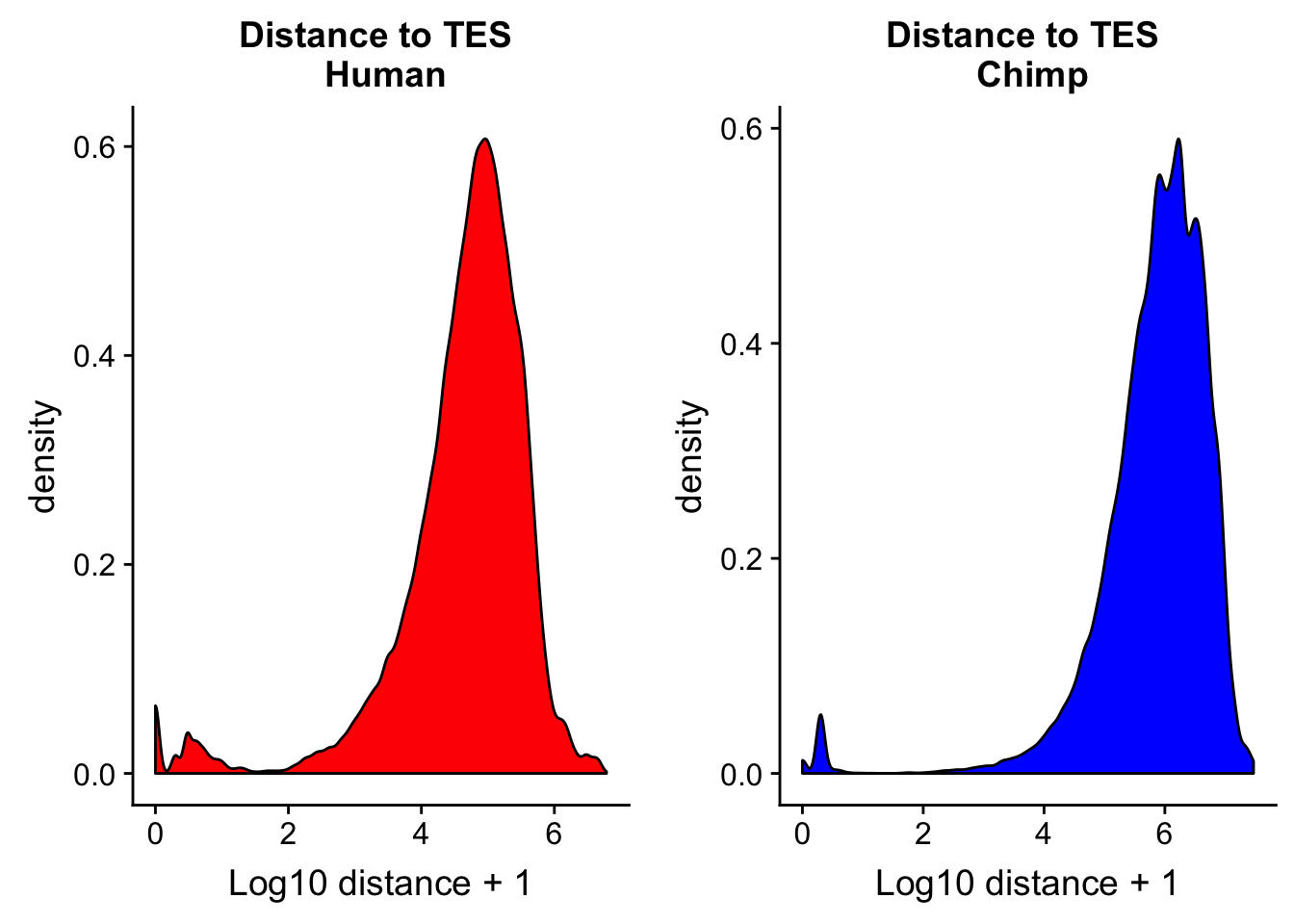

Expand here to see past versions of unnamed-chunk-21-1.png:

Version	Author	Date
1f8f5b1	brimittleman	2018-08-28
a237865	brimittleman	2018-08-24

Flip this and do distance from teh TES to the peak.

#!/bin/bash

#SBATCH --job-name=disTES2Peak
#SBATCH --account=pi-yangili1
#SBATCH --time=24:00:00
#SBATCH --output=disTES2Peak.out
#SBATCH --error=disTES2Peak.err
#SBATCH --partition=broadwl
#SBATCH --mem=12G
#SBATCH --mail-type=END


module load Anaconda3
source activate comp_threeprime_env


bedtools closest -iu -D a -b /project2/gilad/briana/comparitive_threeprime/data/ortho_peaks/humanOrthoPeaks.sort.bed -a /project2/gilad/briana/genome_anotation_data/comp_genomes/gene_annos/humanGene_ncbiRefSeq_TES_sort.bed > /project2/gilad/briana/comparitive_threeprime/data/dist_TES/Human.distTES2Peak.txt

bedtools closest -iu -D a -b /project2/gilad/briana/comparitive_threeprime/data/ortho_peaks/chimpOrthoPeaks.sort.bed  -a /project2/gilad/briana/genome_anotation_data/comp_genomes/gene_annos/chimpGene_refGene_TES_sort.bed > /project2/gilad/briana/comparitive_threeprime/data/dist_TES/Chimp.distTES2Peak.txt

tes2_names=c("genechr", "geneTES_S", "geneTES_E", "gene", "score", "strand", "peakchr", "peakstart", "peakend", "peakname", "dist")
human_TES2dis=read.table("../data/dist_TES/Human.distTES2Peak.txt", stringsAsFactors = F,col.names = tes2_names ) %>% mutate(logdis=log10(abs(dist)+1))

chimp_TES2dist= read.table("../data/dist_TES/Chimp.distTES2Peak.txt", stringsAsFactors = F, col.names = tes2_names) %>% mutate(logdis=log10(abs(dist) + 1))

chTES2=ggplot(chimp_TES2dist, aes(x=logdis)) + geom_density(fill="blue") + labs(title="Distance TES to Peak \n Chimp",x="Log10 distance + 1")

huTES2=ggplot(human_TES2dis, aes(x=logdis)) + geom_density(fill="red") + labs(title="Distance TES to Peak \n Human",x="Log10 distance + 1")


plot_grid(huTES2, chTES2)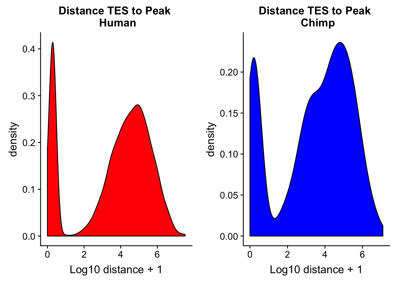

Expand here to see past versions of unnamed-chunk-24-1.png:

Version	Author	Date
1f8f5b1	brimittleman	2018-08-28

Session information

sessionInfo()

R version 3.5.1 (2018-07-02)
Platform: x86_64-apple-darwin15.6.0 (64-bit)
Running under: macOS Sierra 10.12.6

Matrix products: default
BLAS: /Library/Frameworks/R.framework/Versions/3.5/Resources/lib/libRblas.0.dylib
LAPACK: /Library/Frameworks/R.framework/Versions/3.5/Resources/lib/libRlapack.dylib

locale:
[1] en_US.UTF-8/en_US.UTF-8/en_US.UTF-8/C/en_US.UTF-8/en_US.UTF-8

attached base packages:
[1] stats     graphics  grDevices utils     datasets  methods   base     

other attached packages:
 [1] bindrcpp_0.2.2  reshape2_1.4.3  cowplot_0.9.3   workflowr_1.1.1
 [5] forcats_0.3.0   stringr_1.3.1   dplyr_0.7.6     purrr_0.2.5    
 [9] readr_1.1.1     tidyr_0.8.1     tibble_1.4.2    ggplot2_3.0.0  
[13] tidyverse_1.2.1

loaded via a namespace (and not attached):
 [1] tidyselect_0.2.4  haven_1.1.2       lattice_0.20-35  
 [4] colorspace_1.3-2  htmltools_0.3.6   yaml_2.2.0       
 [7] rlang_0.2.2       R.oo_1.22.0       pillar_1.3.0     
[10] glue_1.3.0        withr_2.1.2       R.utils_2.7.0    
[13] modelr_0.1.2      readxl_1.1.0      bindr_0.1.1      
[16] plyr_1.8.4        munsell_0.5.0     gtable_0.2.0     
[19] cellranger_1.1.0  rvest_0.3.2       R.methodsS3_1.7.1
[22] evaluate_0.11     labeling_0.3      knitr_1.20       
[25] broom_0.5.0       Rcpp_0.12.18      scales_1.0.0     
[28] backports_1.1.2   jsonlite_1.5      hms_0.4.2        
[31] digest_0.6.16     stringi_1.2.4     grid_3.5.1       
[34] rprojroot_1.3-2   cli_1.0.0         tools_3.5.1      
[37] magrittr_1.5      lazyeval_0.2.1    crayon_1.3.4     
[40] whisker_0.3-2     pkgconfig_2.0.2   xml2_1.2.0       
[43] lubridate_1.7.4   assertthat_0.2.0  rmarkdown_1.10   
[46] httr_1.3.1        rstudioapi_0.7    R6_2.2.2         
[49] nlme_3.1-137      git2r_0.23.0      compiler_3.5.1

This reproducible R Markdown analysis was created with workflowr 1.1.1