Individaul differences in PAS Usage
Briana Mittleman
2/5/2019
Last updated: 2019-02-25
Checks: 6 0
Knit directory: threeprimeseq/analysis/
This reproducible R Markdown analysis was created with workflowr (version 1.2.0). The Report tab describes the reproducibility checks that were applied when the results were created. The Past versions tab lists the development history.
Great! Since the R Markdown file has been committed to the Git repository, you know the exact version of the code that produced these results.
Great job! The global environment was empty. Objects defined in the global environment can affect the analysis in your R Markdown file in unknown ways. For reproduciblity it’s best to always run the code in an empty environment.
The command set.seed(12345) was run prior to running the code in the R Markdown file. Setting a seed ensures that any results that rely on randomness, e.g. subsampling or permutations, are reproducible.
Great job! Recording the operating system, R version, and package versions is critical for reproducibility.
Nice! There were no cached chunks for this analysis, so you can be confident that you successfully produced the results during this run.
Great! You are using Git for version control. Tracking code development and connecting the code version to the results is critical for reproducibility. The version displayed above was the version of the Git repository at the time these results were generated.
Note that you need to be careful to ensure that all relevant files for the analysis have been committed to Git prior to generating the results (you can use wflow_publish or wflow_git_commit). workflowr only checks the R Markdown file, but you know if there are other scripts or data files that it depends on. Below is the status of the Git repository when the results were generated:
Ignored files:
    Ignored:    .DS_Store
    Ignored:    .Rhistory
    Ignored:    .Rproj.user/
    Ignored:    analysis/figure/
    Ignored:    data/.DS_Store
    Ignored:    data/perm_QTL_trans_noMP_5percov/
    Ignored:    output/.DS_Store

Untracked files:
    Untracked:  KalistoAbundance18486.txt
    Untracked:  analysis/4suDataIGV.Rmd
    Untracked:  analysis/DirectionapaQTL.Rmd
    Untracked:  analysis/EvaleQTLs.Rmd
    Untracked:  analysis/YL_QTL_test.Rmd
    Untracked:  analysis/fixBWChromNames.Rmd
    Untracked:  analysis/groSeqAnalysis.Rmd
    Untracked:  analysis/ncbiRefSeq_sm.sort.mRNA.bed
    Untracked:  analysis/snake.config.notes.Rmd
    Untracked:  analysis/verifyBAM.Rmd
    Untracked:  analysis/verifybam_dubs.Rmd
    Untracked:  code/PeaksToCoverPerReads.py
    Untracked:  code/strober_pc_pve_heatmap_func.R
    Untracked:  data/18486.genecov.txt
    Untracked:  data/APApeaksYL.total.inbrain.bed
    Untracked:  data/AllPeak_counts/
    Untracked:  data/ApaQTLs/
    Untracked:  data/ApaQTLs_otherPhen/
    Untracked:  data/ChromHmmOverlap/
    Untracked:  data/DistTXN2Peak_genelocAnno/
    Untracked:  data/GM12878.chromHMM.bed
    Untracked:  data/GM12878.chromHMM.txt
    Untracked:  data/LianoglouLCL/
    Untracked:  data/LocusZoom/
    Untracked:  data/LocusZoom_proc/
    Untracked:  data/MatchedSnps/
    Untracked:  data/NuclearApaQTLs.txt
    Untracked:  data/PeakCounts/
    Untracked:  data/PeakCounts_noMP_5perc/
    Untracked:  data/PeakCounts_noMP_genelocanno/
    Untracked:  data/PeakUsage/
    Untracked:  data/PeakUsage_noMP/
    Untracked:  data/PeakUsage_noMP_GeneLocAnno/
    Untracked:  data/PeaksUsed/
    Untracked:  data/PeaksUsed_noMP_5percCov/
    Untracked:  data/QTL_overlap/
    Untracked:  data/RNAkalisto/
    Untracked:  data/RefSeq_annotations/
    Untracked:  data/Replicates_usage/
    Untracked:  data/TotalApaQTLs.txt
    Untracked:  data/Totalpeaks_filtered_clean.bed
    Untracked:  data/UnderstandPeaksQC/
    Untracked:  data/WASP_STAT/
    Untracked:  data/YL-SP-18486-T-combined-genecov.txt
    Untracked:  data/YL-SP-18486-T_S9_R1_001-genecov.txt
    Untracked:  data/YL_QTL_test/
    Untracked:  data/apaExamp/
    Untracked:  data/apaExamp_proc/
    Untracked:  data/apaQTL_examp_noMP/
    Untracked:  data/bedgraph_peaks/
    Untracked:  data/bin200.5.T.nuccov.bed
    Untracked:  data/bin200.Anuccov.bed
    Untracked:  data/bin200.nuccov.bed
    Untracked:  data/clean_peaks/
    Untracked:  data/comb_map_stats.csv
    Untracked:  data/comb_map_stats.xlsx
    Untracked:  data/comb_map_stats_39ind.csv
    Untracked:  data/combined_reads_mapped_three_prime_seq.csv
    Untracked:  data/diff_iso_GeneLocAnno/
    Untracked:  data/diff_iso_proc/
    Untracked:  data/diff_iso_trans/
    Untracked:  data/ensemble_to_genename.txt
    Untracked:  data/example_gene_peakQuant/
    Untracked:  data/explainProtVar/
    Untracked:  data/filtPeakOppstrand_cov_noMP_GeneLocAnno_5perc/
    Untracked:  data/filtered_APApeaks_merged_allchrom_refseqTrans.closest2End.bed
    Untracked:  data/filtered_APApeaks_merged_allchrom_refseqTrans.closest2End.noties.bed
    Untracked:  data/first50lines_closest.txt
    Untracked:  data/gencov.test.csv
    Untracked:  data/gencov.test.txt
    Untracked:  data/gencov_zero.test.csv
    Untracked:  data/gencov_zero.test.txt
    Untracked:  data/gene_cov/
    Untracked:  data/joined
    Untracked:  data/leafcutter/
    Untracked:  data/merged_combined_YL-SP-threeprimeseq.bg
    Untracked:  data/molPheno_noMP/
    Untracked:  data/mol_overlap/
    Untracked:  data/mol_pheno/
    Untracked:  data/nom_QTL/
    Untracked:  data/nom_QTL_opp/
    Untracked:  data/nom_QTL_trans/
    Untracked:  data/nuc6up/
    Untracked:  data/nuc_10up/
    Untracked:  data/other_qtls/
    Untracked:  data/pQTL_otherphen/
    Untracked:  data/peakPerRefSeqGene/
    Untracked:  data/perm_QTL/
    Untracked:  data/perm_QTL_GeneLocAnno_noMP_5percov/
    Untracked:  data/perm_QTL_GeneLocAnno_noMP_5percov_3UTR/
    Untracked:  data/perm_QTL_diffWindow/
    Untracked:  data/perm_QTL_opp/
    Untracked:  data/perm_QTL_trans/
    Untracked:  data/perm_QTL_trans_filt/
    Untracked:  data/protAndAPAAndExplmRes.Rda
    Untracked:  data/protAndAPAlmRes.Rda
    Untracked:  data/protAndExpressionlmRes.Rda
    Untracked:  data/reads_mapped_three_prime_seq.csv
    Untracked:  data/smash.cov.results.bed
    Untracked:  data/smash.cov.results.csv
    Untracked:  data/smash.cov.results.txt
    Untracked:  data/smash_testregion/
    Untracked:  data/ssFC200.cov.bed
    Untracked:  data/temp.file1
    Untracked:  data/temp.file2
    Untracked:  data/temp.gencov.test.txt
    Untracked:  data/temp.gencov_zero.test.txt
    Untracked:  data/threePrimeSeqMetaData.csv
    Untracked:  data/threePrimeSeqMetaData55Ind.txt
    Untracked:  data/threePrimeSeqMetaData55Ind.xlsx
    Untracked:  data/threePrimeSeqMetaData55Ind_noDup.txt
    Untracked:  data/threePrimeSeqMetaData55Ind_noDup.xlsx
    Untracked:  data/threePrimeSeqMetaData55Ind_noDup_WASPMAP.txt
    Untracked:  data/threePrimeSeqMetaData55Ind_noDup_WASPMAP.xlsx
    Untracked:  data/~$threePrimeSeqMetaData55Ind_noDup_WASPMAP.xlsx
    Untracked:  output/deeptools_plots/
    Untracked:  output/picard/
    Untracked:  output/plots/
    Untracked:  output/qual.fig2.pdf

Unstaged changes:
    Modified:   analysis/28ind.peak.explore.Rmd
    Modified:   analysis/CompareLianoglouData.Rmd
    Modified:   analysis/NewPeakPostMP.Rmd
    Modified:   analysis/apaQTLoverlapGWAS.Rmd
    Modified:   analysis/cleanupdtseq.internalpriming.Rmd
    Modified:   analysis/coloc_apaQTLs_protQTLs.Rmd
    Modified:   analysis/dif.iso.usage.leafcutter.Rmd
    Modified:   analysis/diffIsoAnalysisNewMapping.Rmd
    Modified:   analysis/diff_iso_pipeline.Rmd
    Modified:   analysis/explainpQTLs.Rmd
    Modified:   analysis/explore.filters.Rmd
    Modified:   analysis/flash2mash.Rmd
    Modified:   analysis/mispriming_approach.Rmd
    Modified:   analysis/overlapMolQTL.Rmd
    Modified:   analysis/overlapMolQTL.opposite.Rmd
    Modified:   analysis/overlap_qtls.Rmd
    Modified:   analysis/peakOverlap_oppstrand.Rmd
    Modified:   analysis/peakQCPPlots.Rmd
    Modified:   analysis/pheno.leaf.comb.Rmd
    Modified:   analysis/pipeline_55Ind.Rmd
    Modified:   analysis/swarmPlots_QTLs.Rmd
    Modified:   analysis/test.max2.Rmd
    Modified:   analysis/test.smash.Rmd
    Modified:   analysis/understandPeaks.Rmd
    Modified:   code/Snakefile
Note that any generated files, e.g. HTML, png, CSS, etc., are not included in this status report because it is ok for generated content to have uncommitted changes.
These are the previous versions of the R Markdown and HTML files. If you’ve configured a remote Git repository (see ?wflow_git_remote), click on the hyperlinks in the table below to view them.
| File | Version | Author | Date | Message |
|---|---|---|---|---|
| Rmd | f1cf46b | Briana Mittleman | 2019-02-25 | account for more metadata |
| html | 4f17cca | Briana Mittleman | 2019-02-15 | Build site. |
| html | d797065 | Briana Mittleman | 2019-02-14 | Build site. |
| Rmd | 3723be9 | Briana Mittleman | 2019-02-14 | fix .8 |
| html | 7b04965 | Briana Mittleman | 2019-02-08 | Build site. |
| Rmd | 4118f08 | Briana Mittleman | 2019-02-08 | add z score |
| html | 39a9453 | Briana Mittleman | 2019-02-07 | Build site. |
| Rmd | 8a106d5 | Briana Mittleman | 2019-02-07 | add all ind heatmap |
| html | 657fb9a | Briana Mittleman | 2019-02-07 | Build site. |
| Rmd | 74276bd | Briana Mittleman | 2019-02-07 | add plot by percentile |
| html | 83ebe13 | Briana Mittleman | 2019-02-07 | Build site. |
| Rmd | e41afd9 | Briana Mittleman | 2019-02-07 | average peak diff by exp and cov |
| html | cc6b1ee | Briana Mittleman | 2019-02-05 | Build site. |
| Rmd | 06912e9 | Briana Mittleman | 2019-02-05 | initiate ind peak usage diff analysis |
library(workflowr)This is workflowr version 1.2.0
Run ?workflowr for help getting startedlibrary(reshape2)
library(matrixStats)
library(tidyverse)── Attaching packages ───────────────────────────────────────────────────────────────────────────────── tidyverse 1.2.1 ──✔ ggplot2 3.0.0 ✔ purrr 0.2.5
✔ tibble 1.4.2 ✔ dplyr 0.7.6
✔ tidyr 0.8.1 ✔ stringr 1.4.0
✔ readr 1.1.1 ✔ forcats 0.3.0Warning: package 'stringr' was built under R version 3.5.2── Conflicts ──────────────────────────────────────────────────────────────────────────────────── tidyverse_conflicts() ──
✖ dplyr::count() masks matrixStats::count()
✖ dplyr::filter() masks stats::filter()
✖ dplyr::lag() masks stats::lag()library(cowplot)
Attaching package: 'cowplot'The following object is masked from 'package:ggplot2':
ggsaveSo far i have been looking at mean peak usage for my filters. As a QC metric, I want to look at the variance in this measurement. I want to understand the reproducibility of the data at a usage percent level. I also want to see if this value is dependent on coverage. I will look at the peaks used in the QTL analysis with 55 individuals and comopute an RNSD value for each gene. This value is computed as \(\sqrt{\sum_{n=1}^N (X-Y)^2}\). Here n is the number of peaks in the gene up to N. X and Y are different individuals. I will plot this value for each gene. I can do this for 2 individuals with low depth and 2 with high depth.
I can start with just the total individuals.
First step is to convert /project2/gilad/briana/threeprimeseq/data/phenotypes_filtPeakTranscript_noMP_GeneLocAnno_5percUs_3UTR/filtered_APApeaks_merged_allchrom_refseqGenes.GeneLocAnno_NoMP_sm_quant.Total.3UTR.fixed.pheno_5perc.fc.gz to numeric.
First I will cut the first column to just get the counts:
less /project2/gilad/briana/threeprimeseq/data/phenotypes_filtPeakTranscript_noMP_GeneLocAnno_5percUs/filtered_APApeaks_merged_allchrom_refseqGenes.GeneLocAnno_NoMP_sm_quant.Total.fixed.pheno_5perc.fc.gz | cut -f1 -d" " --complement | sed '1d' > /project2/gilad/briana/threeprimeseq/data/PeakUsage_noMP_GeneLocAnno/filtered_APApeaks_merged_allchrom_refseqGenes.GeneLocAnno_NoMP_sm_quant.Total.fixed.pheno_5perc.fc_counts 5percCovUsageToNumeric.py
def convert(infile, outfile):
  final=open(outfile, "w")
  for ln in open(infile, "r"):
    line_list=ln.split()
    new_list=[]
    for i in line_list:
      num, dem = i.split("/")
      if dem == "0":
        perc = "0.00"
      else:
        perc = int(num)/int(dem)
        perc=round(perc,2)
        perc= str(perc)
      new_list.append(perc)
    final.write("\t".join(new_list)+ '\n')
  final.close()

convert("/project2/gilad/briana/threeprimeseq/data/PeakUsage_noMP_GeneLocAnno/filtered_APApeaks_merged_allchrom_refseqGenes.GeneLocAnno_NoMP_sm_quant.Total.fixed.pheno_5perc.fc_counts","/project2/gilad/briana/threeprimeseq/data/PeakUsage_noMP_GeneLocAnno/filtered_APApeaks_merged_allchrom_refseqGenes.GeneLocAnno_NoMP_sm_quant.Total.fixed.pheno_5perc.numeric.txt")
Get the gene names from the first file:
less /project2/gilad/briana/threeprimeseq/data/phenotypes_filtPeakTranscript_noMP_GeneLocAnno_5percUs/filtered_APApeaks_merged_allchrom_refseqGenes.GeneLocAnno_NoMP_sm_quant.Total.fixed.pheno_5perc.fc.gz | cut -f1 -d" " | sed '1d' > PeakIDs.txtMerge the files: PeakIDs.txt and the numeric version
paste PeakIDs.txt filtered_APApeaks_merged_allchrom_refseqGenes.GeneLocAnno_NoMP_sm_quant.Total.fixed.pheno_5perc.numeric.txt > filtered_APApeaks_merged_allchrom_refseqGenes.GeneLocAnno_NoMP_sm_quant.Total.fixed.pheno_5perc.numeric.named.txtnames=read.table("../data/PeakUsage_noMP_GeneLocAnno/PeakUsageHeader.txt",stringsAsFactors = F) %>% t %>% as_data_frame()
usageTot=read.table("../data/PeakUsage_noMP_GeneLocAnno/filtered_APApeaks_merged_allchrom_refseqGenes.GeneLocAnno_NoMP_sm_quant.Total.fixed.pheno_5perc.numeric.named.txt", header=F, stringsAsFactors = F)
colnames(usageTot)= names$V1I want to use ind based on coverage
metadataTotal=read.table("../data/threePrimeSeqMetaData55Ind_noDup.txt", header=T) %>% filter(fraction=="total")

#top
metadataTotal %>% arrange(desc(reads)) %>% slice(1:2)
Sample_ID line fraction batch fqlines reads mapped prop_mapped
1 18504_T 18504 total 4 139198896 34799724 25970922 0.7462968
2 18855_T 18855 total 4 139040660 34760165 24532100 0.7057533
Mapped_noMP prop_MappedwithoutMP Sex Wake_Up Collection count1 count2
1 14703998 0.4225320 M 10/31/18 11/19/18 1.9 1.44
2 12999618 0.3739803 F 10/31/18 11/19/18 1.6 1.40
alive1 alive2 alive_avg undiluted_avg Extraction Conentration
1 83 81 82.0 1.67 12.12.18 1984.6
2 71 80 75.5 1.50 12.12.18 2442.9
ratio260_280 to_use h20 threeprime_start Cq cycles library_conc
1 2.07 0.50 9.50 12.17.18 19.67 20 0.402
2 2.08 0.41 9.59 12.17.18 21.00 24 0.353#bottom
metadataTotal %>% arrange(reads) %>% slice(1:2) Sample_ID line fraction batch fqlines reads mapped prop_mapped
1 19160_T 19160 total 2 30319920 7579980 5473593 0.7221118
2 19101_T 19101 total 4 33766300 8441575 6741550 0.7986128
Mapped_noMP prop_MappedwithoutMP Sex Wake_Up Collection count1 count2
1 4009189 0.5289181 M 6/19/18 7/10/18 NA NA
2 3630954 0.4301276 M 11/26/18 12/14/18 0.976 1.05
alive1 alive2 alive_avg undiluted_avg Extraction Conentration
1 NA NA 90 1.100 7.12.18 1287.1
2 76 86 81 1.013 12.16.18 2453.6
ratio260_280 to_use h20 threeprime_start Cq cycles library_conc
1 2.07 0.78 9.22 7.19.18 19.44 20 1.440
2 2.07 0.41 9.59 12.17.18 23.14 24 0.0972 Top read ind: NA18504, NA18855
2 bottom read ind: NA19160, NA19101
topInd=usageTot %>% select(chrom, NA18504, NA18855) %>% separate(chrom, into=c("chr", "start", "end", "geneInf"), sep =":") %>% separate(geneInf, into=c("gene", "strand", "peak"), sep="_") %>% mutate(val=(NA18504-NA18855)^2) %>% group_by(gene) %>% summarise(sumPeaks=sum(val)) %>% mutate(RNSD=sqrt(sumPeaks)) %>% mutate(Sample="Top") %>% select(Sample, RNSD)Warning: Expected 3 pieces. Additional pieces discarded in 3 rows [4917,
4918, 4919].bottomInd=usageTot %>% select(chrom, NA19160, NA19101) %>% separate(chrom, into=c("chr", "start", "end", "geneInf"), sep =":") %>% separate(geneInf, into=c("gene", "strand", "peak"), sep="_") %>% mutate(val=(NA19160-NA19101)^2) %>% group_by(gene) %>% summarise(sumPeaks=sum(val)) %>% mutate(RNSD=sqrt(sumPeaks)) %>% mutate(Sample="Bottom") %>% select(Sample, RNSD)Warning: Expected 3 pieces. Additional pieces discarded in 3 rows [4917,
4918, 4919].bothInd= data.frame(rbind(topInd, bottomInd))ggplot(bothInd, aes(x=RNSD, by=Sample, fill=Sample))+geom_density(alpha=.4) +labs(title="RNSD for peak usage in top 2 and bottom 2 individuals by reads")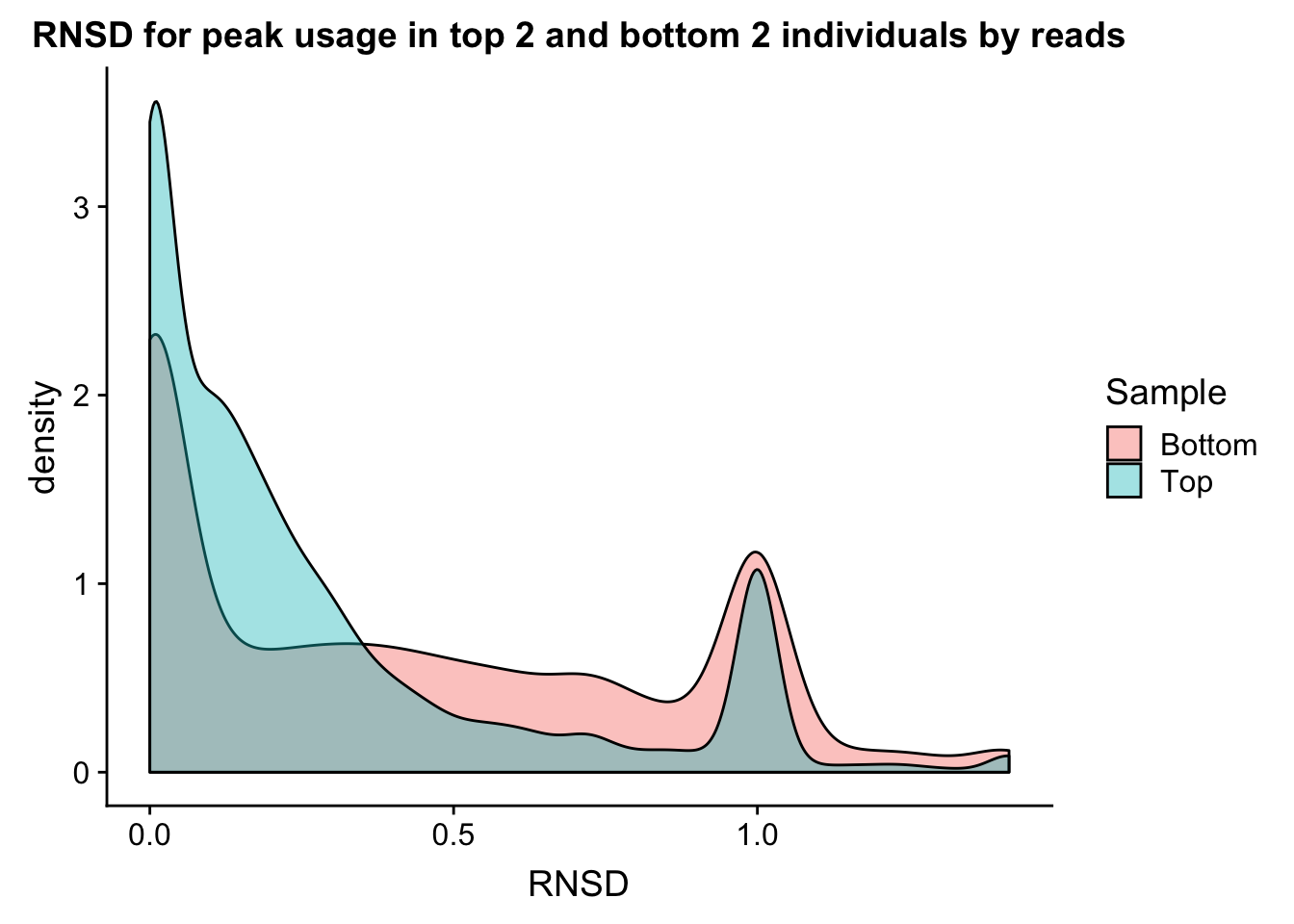
| Version | Author | Date |
|---|---|---|
| 83ebe13 | Briana Mittleman | 2019-02-07 |
ggplot(bothInd, aes(y=RNSD, x=Sample, fill=Sample))+geom_violin() + labs(title="RNSD for peak usage in top 2 and bottom 2 individuals by reads")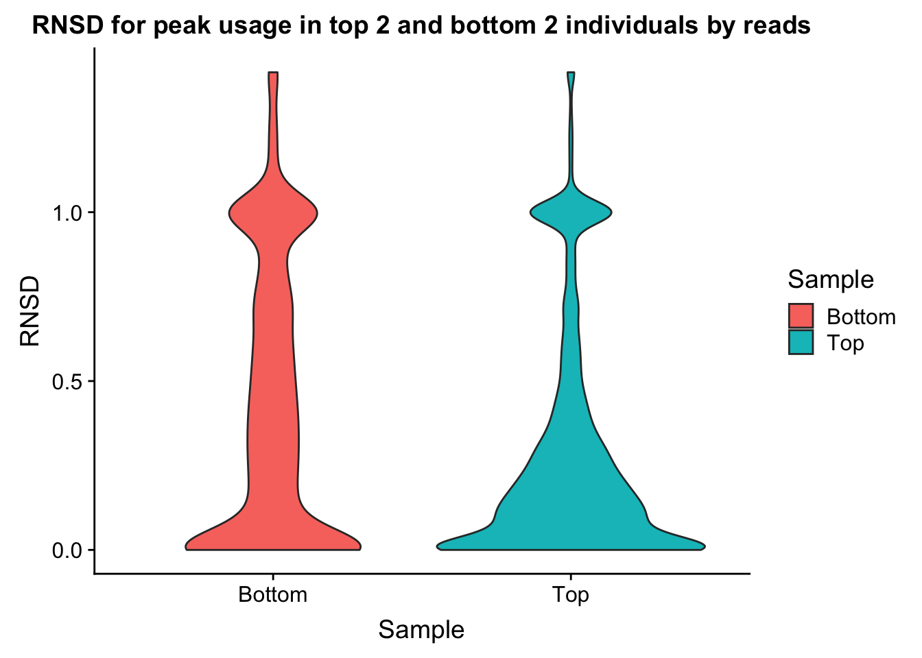
| Version | Author | Date |
|---|---|---|
| 83ebe13 | Briana Mittleman | 2019-02-07 |
Change the statistic to increase the interpretability.
I can look at just genes with 2 peaks. I can then sum the absolute value of the individual differences.
TwoPeakGenes_top= usageTot %>% select(chrom, NA18504, NA18855) %>% separate(chrom, into=c("chr", "start", "end", "geneInf"), sep =":") %>% separate(geneInf, into=c("gene", "strand", "peak"), sep="_") %>% group_by(gene) %>% mutate(nPeak=n()) %>% filter(nPeak==2)Warning: Expected 3 pieces. Additional pieces discarded in 3 rows [4917,
4918, 4919].n2Peak=unique(TwoPeakGenes_top$gene) %>% length() This gives us 3448 genes.
TwoPeakGenes_top_stat= TwoPeakGenes_top %>% mutate(absDiff=abs(NA18504-NA18855)) %>% group_by(gene) %>% select(gene, absDiff) %>% distinct(gene, .keep_all=T)
Avg2PeakGeneTop=sum(TwoPeakGenes_top_stat$absDiff)/n2Peak
Avg2PeakGeneTop
[1] 0.1994083Now do this for the bottom 2 ind:
TwoPeakGenes_bottom= usageTot %>% select(chrom, NA19160, NA19101) %>% separate(chrom, into=c("chr", "start", "end", "geneInf"), sep =":") %>% separate(geneInf, into=c("gene", "strand", "peak"), sep="_") %>% group_by(gene) %>% mutate(nPeak=n()) %>% filter(nPeak==2)Warning: Expected 3 pieces. Additional pieces discarded in 3 rows [4917,
4918, 4919].TwoPeakGenes_bottom_stat= TwoPeakGenes_bottom %>% mutate(absDiff=abs(NA19101-NA19160)) %>% group_by(gene) %>% select(gene, absDiff) %>% distinct(gene, .keep_all=T)
Avg2PeakGeneBottom=sum(TwoPeakGenes_bottom_stat$absDiff)/n2Peak
Avg2PeakGeneBottom[1] 0.2874909This demonstrates we may have some noise in the data and have not reached sequencing saturation. However, this could be driven by lowly expressed genes. I will fraction this analysis by the top expressed and bottom expressed genes. To do this I will pull in the count data (before we had usage parameters) and add to this table the mean counts.
Count files:
- /project2/gilad/briana/threeprimeseq/data/filtPeakOppstrand_cov_noMP_GeneLocAnno/filtered_APApeaks_merged_allchrom_refseqGenes.GeneLocAnno_NoMP_sm_quant.Nuclear.fixed.fc
- /project2/gilad/briana/threeprimeseq/data/filtPeakOppstrand_cov_noMP_GeneLocAnno/filtered_APApeaks_merged_allchrom_refseqGenes.GeneLocAnno_NoMP_sm_quant.Total.fixed.fc
I need to filter these for the peaks I kept after the 5% usage filter.
filterCounts_5percCovPeaks.py
#python

totalokPeaks5perc_file="/project2/gilad/briana/threeprimeseq/data/phenotypes_filtPeakTranscript_noMP_GeneLocAnno/filtered_APApeaks_merged_allchrom_refseqGenes.GeneLocAnno.NoMP_sm_quant.Total_fixed.pheno.5percPeaks.txt"

totalokPeaks5perc={}
for ln in open(totalokPeaks5perc_file,"r"):
    peakname=ln.split()[5]
    totalokPeaks5perc[peakname]=""


nuclearokPeaks5perc_file="/project2/gilad/briana/threeprimeseq/data/phenotypes_filtPeakTranscript_noMP_GeneLocAnno/filtered_APApeaks_merged_allchrom_refseqGenes.GeneLocAnno.NoMP_sm_quant.Nuclear_fixed.pheno.5percPeaks.txt"
nuclearokPeaks5perc={}
for ln in open(nuclearokPeaks5perc_file,"r"):
    peakname=ln.split()[5]
    nuclearokPeaks5perc[peakname]=""


totalPhenoBefore=open("/project2/gilad/briana/threeprimeseq/data/filtPeakOppstrand_cov_noMP_GeneLocAnno/filtered_APApeaks_merged_allchrom_refseqGenes.GeneLocAnno_NoMP_sm_quant.Total.fixed.fc","r")
totalPhenoAfter=open("/project2/gilad/briana/threeprimeseq/data/filtPeakOppstrand_cov_noMP_GeneLocAnno_5perc/filtered_APApeaks_merged_allchrom_refseqGenes.GeneLocAnno_NoMP_sm_quant.Total.fixed.5perc.fc", "w")
for num, ln in enumerate(totalPhenoBefore):
    if num == 1:
        totalPhenoAfter.write(ln)
    if num >1:
        id=ln.split()[0].split(":")[0]
        if id in totalokPeaks5perc.keys():
            totalPhenoAfter.write(ln)
totalPhenoAfter.close()

nuclearPhenoBefore=open("/project2/gilad/briana/threeprimeseq/data/filtPeakOppstrand_cov_noMP_GeneLocAnno/filtered_APApeaks_merged_allchrom_refseqGenes.GeneLocAnno_NoMP_sm_quant.Nuclear.fixed.fc","r")
nuclearPhenoAfter=open("/project2/gilad/briana/threeprimeseq/data/filtPeakOppstrand_cov_noMP_GeneLocAnno_5perc/filtered_APApeaks_merged_allchrom_refseqGenes.GeneLocAnno_NoMP_sm_quant.Nuclear.fixed.5perc.fc", "w")
for num, ln in enumerate(nuclearPhenoBefore):
    if num ==1:
        nuclearPhenoAfter.write(ln)
    if num > 1:
        id=ln.split()[0].split(":")[0]
        if id in nuclearokPeaks5perc.keys():
            nuclearPhenoAfter.write(ln)
nuclearPhenoAfter.close()
Pull the filtered counts for the total here and get the genes in TwoPeakGenes_top_stat$gene. For simplicity I will just look at the ind. with the top coverage.
TotalCounts=read.table("../data/filtPeakOppstrand_cov_noMP_GeneLocAnno_5perc/filtered_APApeaks_merged_allchrom_refseqGenes.GeneLocAnno_NoMP_sm_quant.Total.fixed.5perc.fc", header=T, stringsAsFactors = F) %>% separate(Geneid, into =c('peak', 'chr', 'start', 'end', 'strand', 'gene'), sep = ":") %>% select(-peak, -chr, -start, -end, -strand, -Chr, -Start, -End, -Strand, -Length) %>% group_by(gene) %>% mutate(PeakCount=n()) %>% filter(PeakCount==2) %>% select(gene, X18504_T) %>% group_by(gene) %>% summarise(Exp=sum(X18504_T)) Top 1000 genes
TotalCounts_top1000= TotalCounts %>% arrange(desc(Exp)) %>% top_n(1000)Selecting by ExpJoin this with top ind:
TwoPeakGenes_top_stat_top100 = TwoPeakGenes_top_stat %>% inner_join(TotalCounts_top1000, by="gene")

Avg2PeakGeneTopExpHigh=sum(TwoPeakGenes_top_stat_top100$absDiff)/nrow(TwoPeakGenes_top_stat_top100)
Avg2PeakGeneTopExpHigh
[1] 0.1043955Do the same for low expressed genes (not 0)
TotalCounts_bottom1000= TotalCounts %>% filter(Exp > 0) %>% top_n(-1000)Selecting by ExpTwoPeakGenes_top_stat_bottom100 = TwoPeakGenes_top_stat %>% inner_join(TotalCounts_bottom1000, by="gene")
Avg2PeakGeneTopExpLow=sum(TwoPeakGenes_top_stat_bottom100$absDiff)/nrow(TwoPeakGenes_top_stat_bottom100)
Avg2PeakGeneTopExpLow[1] 0.3264855Do this for the other individuals as wel..
TwoPeakGenes_bottom_stat_top100 = TwoPeakGenes_bottom_stat %>% inner_join(TotalCounts_top1000, by="gene")

Avg2PeakGeneBottomExpHigh=sum(TwoPeakGenes_bottom_stat_top100$absDiff)/nrow(TwoPeakGenes_bottom_stat_top100)
Avg2PeakGeneBottomExpHigh
[1] 0.2012343TwoPeakGenes_bottom_stat_bottom100 = TwoPeakGenes_bottom_stat %>% inner_join(TotalCounts_bottom1000, by="gene")
Avg2PeakGeneBottomExpLow=sum(TwoPeakGenes_bottom_stat_bottom100$absDiff)/nrow(TwoPeakGenes_bottom_stat_bottom100)
Avg2PeakGeneBottomExpLow[1] 0.3691848Make a plot with these values:
avgPeakUsageTable=data.frame(rbind(c("Top", "High", .1), c("Top", "Low", .32), c("Bottom", "High", .19), c("Bottom", "Low", .35)))
colnames(avgPeakUsageTable)= c("Coverage", "Expression", "AverageUsageDiff")
ggplot(avgPeakUsageTable,aes(y=AverageUsageDiff, x=Coverage, by=Expression, fill=Expression)) + geom_bar(stat="identity",position="dodge") + labs(title="Difference between individual usage \ndepends on expression and coverage")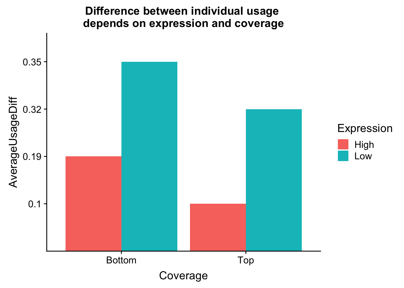
I want to look at this based on every 10% of gene expression. First I will remove genes with 0 coverage in this ind.
TotalCounts_no0=TotalCounts %>% filter(Exp>0)
nrow(TotalCounts_no0)
[1] 3143I can add a column that is the rank over the sum (or the percentile)
TotalCounts_no0_perc= TotalCounts_no0 %>% mutate(Percentile = percent_rank(Exp)) TotalCounts_no0_perc10= TotalCounts_no0_perc %>% filter(Percentile<.1)
TotalCounts_no0_perc20= TotalCounts_no0_perc %>% filter(Percentile<.2, Percentile>.1)
TotalCounts_no0_perc30= TotalCounts_no0_perc %>% filter(Percentile<.3, Percentile>.2)
TotalCounts_no0_perc40= TotalCounts_no0_perc %>% filter(Percentile<.4, Percentile>.3)
TotalCounts_no0_perc50= TotalCounts_no0_perc %>% filter(Percentile<.5, Percentile>.4)
TotalCounts_no0_perc60= TotalCounts_no0_perc %>% filter(Percentile<.6, Percentile>.5)
TotalCounts_no0_perc70= TotalCounts_no0_perc %>% filter(Percentile<.7, Percentile>.6)
TotalCounts_no0_perc80= TotalCounts_no0_perc %>% filter(Percentile<8, Percentile>.7)
TotalCounts_no0_perc90= TotalCounts_no0_perc %>% filter(Percentile<.9, Percentile>.8)
TotalCounts_no0_perc100= TotalCounts_no0_perc %>% filter(Percentile<1, Percentile>.9)Now I can make a function that takes one of these files, and computes the relevant stat. This takes the usage file and the expression file
getAvgDiffUsage=function(Usage, exp){
  df = Usage %>% inner_join(exp, by="gene")
  value=df=sum(df$absDiff)/nrow(df)
  return(value)
}
Run this for the top coverage at each exp:
AvgUsageDiff_top10=getAvgDiffUsage(TwoPeakGenes_top_stat, exp=TotalCounts_no0_perc10)
AvgUsageDiff_top20=getAvgDiffUsage(TwoPeakGenes_top_stat, exp=TotalCounts_no0_perc20)
AvgUsageDiff_top30=getAvgDiffUsage(TwoPeakGenes_top_stat, exp=TotalCounts_no0_perc30)
AvgUsageDiff_top40=getAvgDiffUsage(TwoPeakGenes_top_stat, exp=TotalCounts_no0_perc40)
AvgUsageDiff_top50=getAvgDiffUsage(TwoPeakGenes_top_stat, exp=TotalCounts_no0_perc50)
AvgUsageDiff_top60=getAvgDiffUsage(TwoPeakGenes_top_stat, exp=TotalCounts_no0_perc60)
AvgUsageDiff_top70=getAvgDiffUsage(TwoPeakGenes_top_stat, exp=TotalCounts_no0_perc70)
AvgUsageDiff_top80=getAvgDiffUsage(TwoPeakGenes_top_stat, exp=TotalCounts_no0_perc80)
AvgUsageDiff_top90=getAvgDiffUsage(TwoPeakGenes_top_stat, exp=TotalCounts_no0_perc90)
AvgUsageDiff_top100=getAvgDiffUsage(TwoPeakGenes_top_stat, exp=TotalCounts_no0_perc100)

AvgUsageTop=c(AvgUsageDiff_top10,AvgUsageDiff_top20,AvgUsageDiff_top30,AvgUsageDiff_top40,AvgUsageDiff_top50,AvgUsageDiff_top60,AvgUsageDiff_top70,AvgUsageDiff_top80,AvgUsageDiff_top90,AvgUsageDiff_top100)
Do this for Bottom coverage:
AvgUsageDiff_bottom10=getAvgDiffUsage(TwoPeakGenes_bottom_stat, exp=TotalCounts_no0_perc10)
AvgUsageDiff_bottom20=getAvgDiffUsage(TwoPeakGenes_bottom_stat, exp=TotalCounts_no0_perc20)
AvgUsageDiff_bottom30=getAvgDiffUsage(TwoPeakGenes_bottom_stat, exp=TotalCounts_no0_perc30)
AvgUsageDiff_bottom40=getAvgDiffUsage(TwoPeakGenes_bottom_stat, exp=TotalCounts_no0_perc40)
AvgUsageDiff_bottom50=getAvgDiffUsage(TwoPeakGenes_bottom_stat, exp=TotalCounts_no0_perc50)
AvgUsageDiff_bottom60=getAvgDiffUsage(TwoPeakGenes_bottom_stat, exp=TotalCounts_no0_perc60)
AvgUsageDiff_bottom70=getAvgDiffUsage(TwoPeakGenes_bottom_stat, exp=TotalCounts_no0_perc70)
AvgUsageDiff_bottom80=getAvgDiffUsage(TwoPeakGenes_bottom_stat, exp=TotalCounts_no0_perc80)
AvgUsageDiff_bottom90=getAvgDiffUsage(TwoPeakGenes_bottom_stat, exp=TotalCounts_no0_perc90)
AvgUsageDiff_bottom100=getAvgDiffUsage(TwoPeakGenes_bottom_stat, exp=TotalCounts_no0_perc100)

AvgUsagebottom=c(AvgUsageDiff_bottom10,AvgUsageDiff_bottom20,AvgUsageDiff_bottom30,AvgUsageDiff_bottom40,AvgUsageDiff_bottom50,AvgUsageDiff_bottom60,AvgUsageDiff_bottom70,AvgUsageDiff_bottom80,AvgUsageDiff_bottom90,AvgUsageDiff_bottom100)
All together:
Percentile=c(10,20,30,40,50,60,70,80,90,100)
allAvgUsage=data.frame(cbind(Percentile,AvgUsageTop,AvgUsagebottom))
colnames(allAvgUsage)=c("Percentile","Top", "Bottom")
allAvgUsage$Top= as.numeric(as.character(allAvgUsage$Top))
allAvgUsage$Bottom= as.numeric(as.character(allAvgUsage$Bottom))
allAvgUsage_melt= melt(allAvgUsage, id.vars = c("Percentile"))
colnames(allAvgUsage_melt)=c("Percentile","Coverage", "AvgDifference")
ggplot(allAvgUsage_melt, aes(x=Percentile, y=AvgDifference,by=Coverage, fill=Coverage)) + geom_bar(stat="identity", position = "dodge") + labs(title="Average Usage Difference between 2 individauls by 3' Seq \nCount percentile and coverage") + scale_x_discrete(limits = c(10,20,30,40,50,60,70,80,90,100))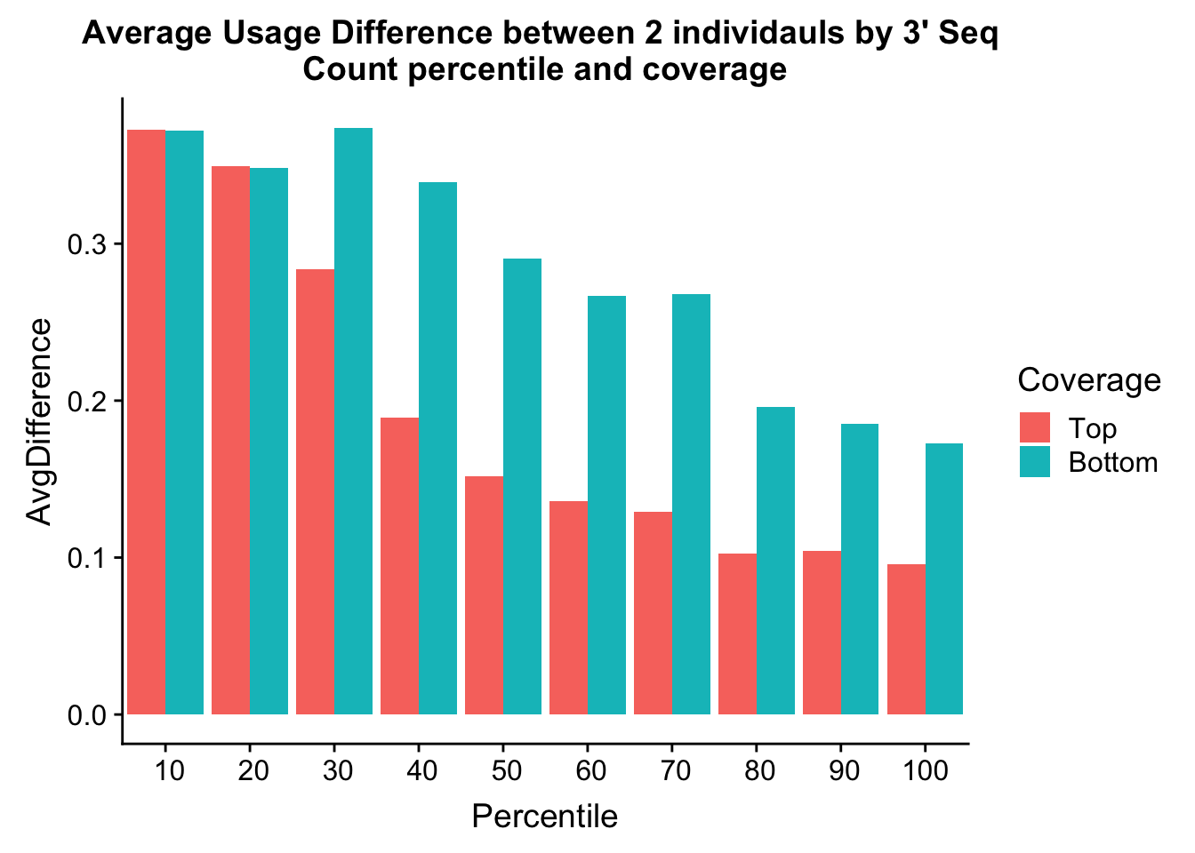
| Version | Author | Date |
|---|---|---|
| 657fb9a | Briana Mittleman | 2019-02-07 |
Total counts for a low coverage individual:
TotalCounts_low=read.table("../data/filtPeakOppstrand_cov_noMP_GeneLocAnno_5perc/filtered_APApeaks_merged_allchrom_refseqGenes.GeneLocAnno_NoMP_sm_quant.Total.fixed.5perc.fc", header=T, stringsAsFactors = F) %>% separate(Geneid, into =c('peak', 'chr', 'start', 'end', 'strand', 'gene'), sep = ":") %>% select(-peak, -chr, -start, -end, -strand, -Chr, -Start, -End, -Strand, -Length) %>% group_by(gene) %>% mutate(PeakCount=n()) %>% filter(PeakCount==2) %>% select(gene, X19101_T) %>% group_by(gene) %>% summarise(Exp=sum(X19101_T))
TotalCounts_no0_low=TotalCounts_low %>% filter(Exp>0)
TotalCounts_no0_perc_low= TotalCounts_no0_low %>% mutate(Percentile = percent_rank(Exp))
This will be more informative if we do 1 vs all. Now instead of Y being 1 individual it is the average of all other individuals at that peak. I will make a heatmap with y as the individual and x as the percentile.
I need to create a function that can take in an individual, removes it from the matrix. computes the mean for the other individuals then merges the numbers back together, it will then compute the values for each percentile as I did before and returns a list of the averageUsageDifferences. I need to compute the percentile for the individual
Input dataframe with usage values for genes with only 2 peaks.
usageTot_2peak= usageTot %>% separate(chrom, into=c("chr", "start", "end", "geneInf"), sep =":") %>% separate(geneInf, into=c("gene", "strand", "peak"), sep="_") %>% group_by(gene) %>% mutate(nPeak=n()) %>% filter(nPeak==2) %>% select(-chr, -start, -end, -strand, -peak, -nPeak) %>% ungroup()Warning: Expected 3 pieces. Additional pieces discarded in 3 rows [4917,
4918, 4919].TotalCounts_AllInd=read.table("../data/filtPeakOppstrand_cov_noMP_GeneLocAnno_5perc/filtered_APApeaks_merged_allchrom_refseqGenes.GeneLocAnno_NoMP_sm_quant.Total.fixed.5perc.fc", header=T, stringsAsFactors = F) %>% separate(Geneid, into =c('peak', 'chr', 'start', 'end', 'strand', 'gene'), sep = ":") %>% select(-peak, -chr, -start, -end, -strand, -Chr, -Start, -End, -Strand, -Length) %>% group_by(gene) %>% mutate(PeakCount=n()) %>% filter(PeakCount==2) %>% select(-PeakCount) %>% ungroup()
colnames(TotalCounts_AllInd)=colnames(usageTot_2peak)This will take tidy eval because my
perIndDiffUsage=function(ind, counts=TotalCounts_AllInd, usage=usageTot_2peak){
  ind=enquo(ind)
  #compute usage stats
  #seperate usage
  usage_ind=usage %>% select(gene, !!ind)
  usage_other = usage %>% select(-gene,-!!ind) %>% rowMeans()
  usage_indVal=as.data.frame(cbind(usage_ind,usage_other))
  usage_indVal$val=abs(usage_indVal[,2] - usage_indVal[,3])
  usage_indVal2= usage_indVal%>% group_by(gene) %>% select(gene, val) %>% distinct(gene, .keep_all=T)
  #seperate genes by percentile for this ind
  count_ind= counts %>% select(gene, !!ind)
  colnames(count_ind)=c("gene", "count")
  count_ind = count_ind %>%  group_by(gene) %>% summarize(Exp=sum(count)) %>% filter(Exp >0)  %>% mutate(Percentile = percent_rank(Exp))
  count_ind_perc10= count_ind %>% filter(Percentile<.1)
  count_ind_perc20= count_ind %>% filter(Percentile<.2, Percentile>.1)
  count_ind_perc30= count_ind %>% filter(Percentile<.3, Percentile>.2)
  count_ind_perc40= count_ind %>% filter(Percentile<.4, Percentile>.3)
  count_ind_perc50= count_ind %>% filter(Percentile<.5, Percentile>.4)
  count_ind_perc60= count_ind %>% filter(Percentile<.6, Percentile>.5)
  count_ind_perc70= count_ind %>% filter(Percentile<.7, Percentile>.6)
  count_ind_perc80= count_ind %>% filter(Percentile<.8, Percentile>.7)
  count_ind_perc90= count_ind %>% filter(Percentile<.9, Percentile>.8)
  count_ind_perc100= count_ind %>% filter(Percentile<1, Percentile>.9)
  #subset and sum usage
  out10_df= usage_indVal2 %>% inner_join(count_ind_perc10, by="gene")
  out20_df= usage_indVal2 %>% inner_join(count_ind_perc20, by="gene")
  out30_df= usage_indVal2 %>% inner_join(count_ind_perc30, by="gene")
  out40_df= usage_indVal2 %>% inner_join(count_ind_perc40, by="gene")
  out50_df= usage_indVal2 %>% inner_join(count_ind_perc50, by="gene")
  out60_df= usage_indVal2 %>% inner_join(count_ind_perc60, by="gene")
  out70_df= usage_indVal2 %>% inner_join(count_ind_perc70, by="gene")
  out80_df= usage_indVal2 %>% inner_join(count_ind_perc80, by="gene")
  out90_df= usage_indVal2 %>% inner_join(count_ind_perc90, by="gene")
  out100_df= usage_indVal2 %>% inner_join(count_ind_perc100, by="gene")
  #output list of 10 values
  out= c((sum(out10_df$val)/nrow(out10_df)), (sum(out20_df$val)/nrow(out20_df)), (sum(out30_df$val)/nrow(out30_df)), (sum(out40_df$val)/nrow(out40_df)), (sum(out50_df$val)/nrow(out50_df)), (sum(out60_df$val)/nrow(out60_df)), (sum(out70_df$val)/nrow(out70_df)), (sum(out80_df$val)/nrow(out80_df)), (sum(out90_df$val)/nrow(out90_df)), (sum(out100_df$val)/nrow(out100_df)))
  return(out)
}
Run this function for each individual and append the result to a df:
Inds=colnames(TotalCounts_AllInd)[2:ncol(TotalCounts_AllInd)]
Percentile=c(10,20,30,40,50,60,70,80,90,100)
for (i in Inds){
  x= perIndDiffUsage(i)
  Percentile=cbind(Percentile, x)
}
colnames(Percentile)=c("Percentile", Inds)
Lineorder=metadataTotal %>% arrange(desc(reads)) %>% select(line) %>% mutate(sample=paste("NA" , line, sep=""))
Lineorder=Lineorder$sample
Percentile_df=as.data.frame(Percentile) %>% select(Percentile, Lineorder)
#order the
Percentile_melt=melt(Percentile_df, id.vars=c("Percentile"))
colnames(Percentile_melt)=c("Percentile", "Individual", "AvgUsageDiff")Plot this:
ggplot(Percentile_melt, aes(x=Percentile, y=Individual, fill=AvgUsageDiff)) + geom_tile() + labs(title="Average peak usage difference for individaul vs. others \n by percentile of gene counts arranged by reads counts") + scale_fill_gradientn(colours = c("white", "red", "black"))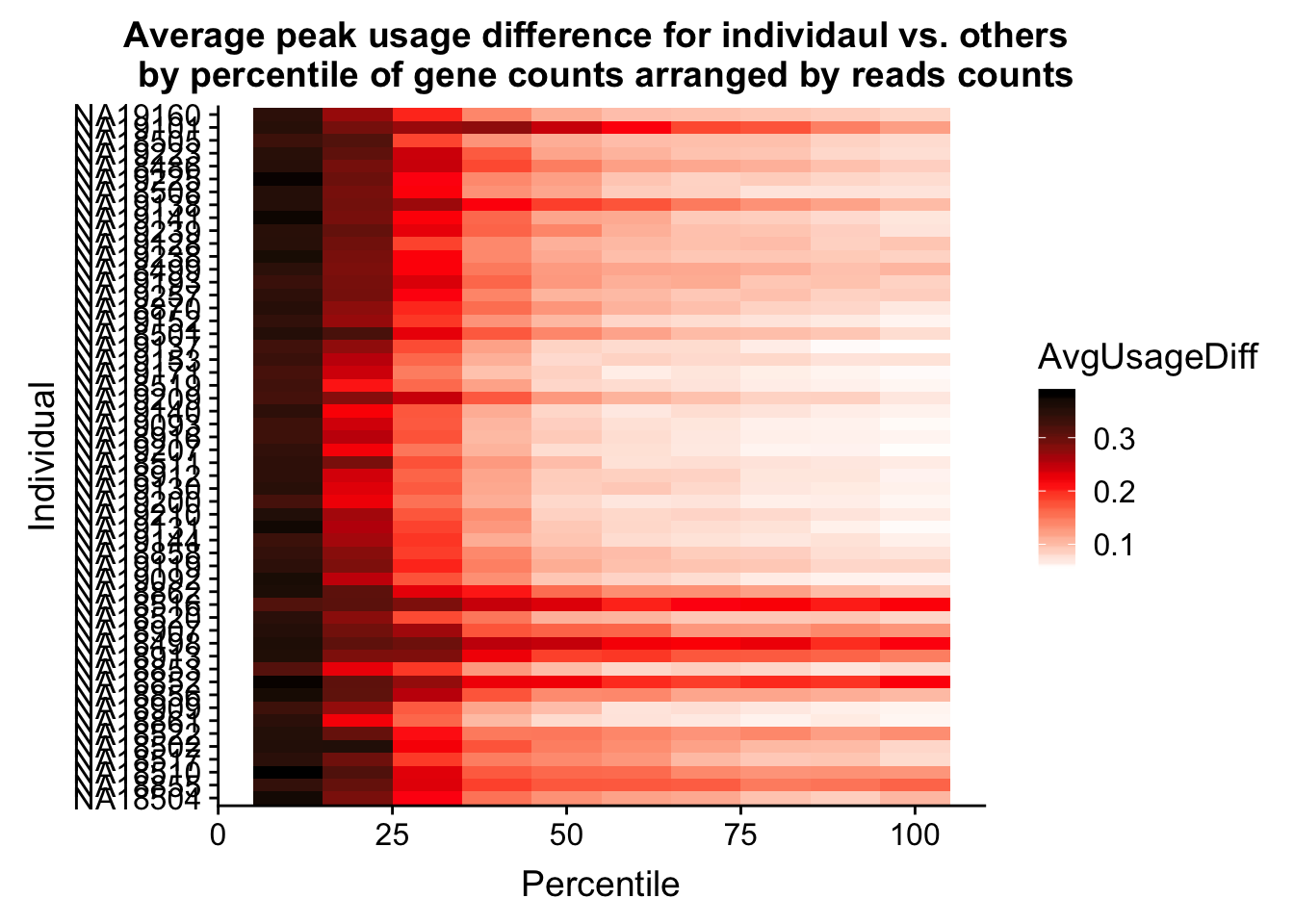
Lineorder_map=metadataTotal %>% arrange(desc(Mapped_noMP))  %>% select(line) %>% mutate(sample=paste("NA" , line, sep=""))
Lineorder_map=Lineorder_map$sample

Percentile_df2=as.data.frame(Percentile) %>%   select(Percentile, Lineorder_map)

#order the

Percentile_melt2=melt(Percentile_df2, id.vars=c("Percentile"))
colnames(Percentile_melt2)=c("Percentile", "Individual", "AvgUsageDiff")

ggplot(Percentile_melt2, aes(x=Percentile, y=Individual, fill=AvgUsageDiff)) + geom_tile() + labs(title="Average peak usage difference for individaul vs. others \n by percentile of gene counts arranged by mapped reads counts") + scale_fill_gradientn(colours = c("white", "red", "black"))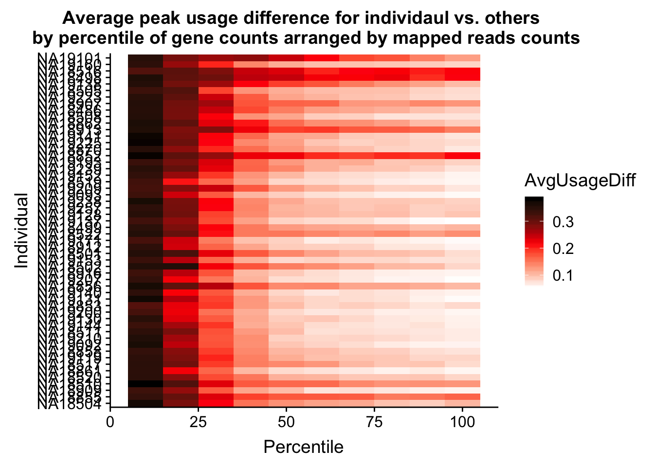
Try this again but with Z scores. I will get the mean and SD for each peak and compute the |x-mean|/sd
perIndDiffUsage_Z=function(ind, counts=TotalCounts_AllInd, usage=usageTot_2peak){
  ind=enquo(ind)
  #compute usage stats
  #seperate usage
  usage_ind=usage %>% select(gene, !!ind)
  usage_mean = usage %>% select(-gene) %>% rowMeans()
  usage_df=usage %>% select(-gene)
  usage_sd= as.matrix(usage_df)%>% rowSds()
  usage_indVal=as.data.frame(cbind(usage_ind,usage_mean, usage_sd))
  usage_indVal$val=abs(usage_indVal[,2] - usage_indVal[,3])/usage_indVal[,4]
  usage_indVal2= usage_indVal%>% group_by(gene) %>% select(gene, val) %>% distinct(gene, .keep_all=T)
  #seperate genes by percentile for this ind
  count_ind= counts %>% select(gene, !!ind)
  colnames(count_ind)=c("gene", "count")
  count_ind = count_ind %>%  group_by(gene) %>% summarize(Exp=sum(count)) %>% filter(Exp >0)  %>% mutate(Percentile = percent_rank(Exp))
  count_ind_perc10= count_ind %>% filter(Percentile<.1)
  count_ind_perc20= count_ind %>% filter(Percentile<.2, Percentile>.1)
  count_ind_perc30= count_ind %>% filter(Percentile<.3, Percentile>.2)
  count_ind_perc40= count_ind %>% filter(Percentile<.4, Percentile>.3)
  count_ind_perc50= count_ind %>% filter(Percentile<.5, Percentile>.4)
  count_ind_perc60= count_ind %>% filter(Percentile<.6, Percentile>.5)
  count_ind_perc70= count_ind %>% filter(Percentile<.7, Percentile>.6)
  count_ind_perc80= count_ind %>% filter(Percentile<.8, Percentile>.7)
  count_ind_perc90= count_ind %>% filter(Percentile<.9, Percentile>.8)
  count_ind_perc100= count_ind %>% filter(Percentile<1, Percentile>.9)
  #subset and sum usage
  out10_df= usage_indVal2 %>% inner_join(count_ind_perc10, by="gene")
  out20_df= usage_indVal2 %>% inner_join(count_ind_perc20, by="gene")
  out30_df= usage_indVal2 %>% inner_join(count_ind_perc30, by="gene")
  out40_df= usage_indVal2 %>% inner_join(count_ind_perc40, by="gene")
  out50_df= usage_indVal2 %>% inner_join(count_ind_perc50, by="gene")
  out60_df= usage_indVal2 %>% inner_join(count_ind_perc60, by="gene")
  out70_df= usage_indVal2 %>% inner_join(count_ind_perc70, by="gene")
  out80_df= usage_indVal2 %>% inner_join(count_ind_perc80, by="gene")
  out90_df= usage_indVal2 %>% inner_join(count_ind_perc90, by="gene")
  out100_df= usage_indVal2 %>% inner_join(count_ind_perc100, by="gene")
  #output list of 10 values
  out= c((sum(out10_df$val)/nrow(out10_df)), (sum(out20_df$val)/nrow(out20_df)), (sum(out30_df$val)/nrow(out30_df)), (sum(out40_df$val)/nrow(out40_df)), (sum(out50_df$val)/nrow(out50_df)), (sum(out60_df$val)/nrow(out60_df)), (sum(out70_df$val)/nrow(out70_df)), (sum(out80_df$val)/nrow(out80_df)), (sum(out90_df$val)/nrow(out90_df)), (sum(out100_df$val)/nrow(out100_df)))
  return(out)
}
Inds=colnames(TotalCounts_AllInd)[2:ncol(TotalCounts_AllInd)]
Percentile_z=c(10,20,30,40,50,60,70,80,90,100)
for (i in Inds){
x= perIndDiffUsage_Z(i)
Percentile_z=cbind(Percentile_z, x)
}
colnames(Percentile_z)=c("Percentile", Inds)Percentile_z_df=as.data.frame(Percentile_z) %>% select(Percentile, Lineorder)
#order the
Percentile_z_melt=melt(Percentile_z_df, id.vars=c("Percentile"))
colnames(Percentile_z_melt)=c("Percentile", "Individual", "AvgUsageDiff")
ggplot(Percentile_z_melt, aes(x=Percentile, y=Individual, fill=AvgUsageDiff)) + geom_tile() + labs(title="Peak usage difference Z score for individaul vs. others \n by percentile of gene counts arranged by reads counts") + scale_fill_gradientn(colours = c("white", "red", "black"))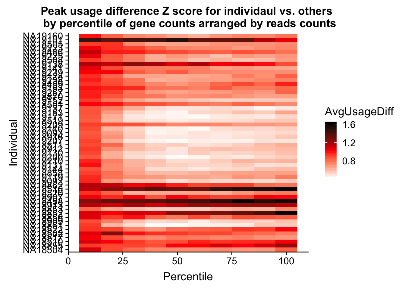
Do this by the mapped reads:
Percentile_z_df2=as.data.frame(Percentile_z) %>%   select(Percentile, Lineorder_map)

#order the

Percentile_z_melt2=melt(Percentile_z_df2, id.vars=c("Percentile"))
colnames(Percentile_z_melt2)=c("Percentile", "Individual", "AvgUsageDiff")

ggplot(Percentile_z_melt2, aes(x=Percentile, y=Individual, fill=AvgUsageDiff)) + geom_tile() + labs(title="Peak usage difference Z score for individaul vs. others \n by percentile of gene counts arranged by mapped reads counts") + scale_fill_gradientn(colours = c("white", "red", "black"))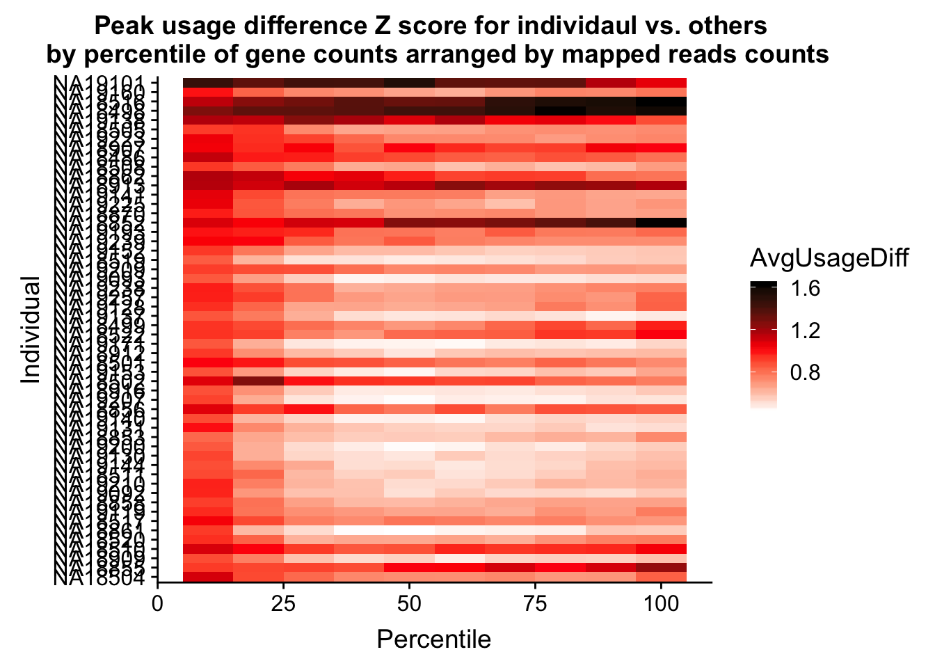
Try ordering this by library concentration:
concentration=metadataTotal %>% arrange(desc(library_conc)) %>% select(line) %>% mutate(sample=paste("NA" , line, sep=""))
concentration=concentration$sample
Percentile_df_conc=as.data.frame(Percentile) %>% select(Percentile, concentration)
#order the
Percentile_conc_melt=melt(Percentile_df_conc, id.vars=c("Percentile"))
colnames(Percentile_conc_melt)=c("Percentile", "Individual", "AvgUsageDiff")
ggplot(Percentile_conc_melt, aes(x=Percentile, y=Individual, fill=AvgUsageDiff)) + geom_tile() + labs(title="Average peak usage difference for individaul vs. others \n by lib conc ") + scale_fill_gradientn(colours = c("white", "red", "black")) 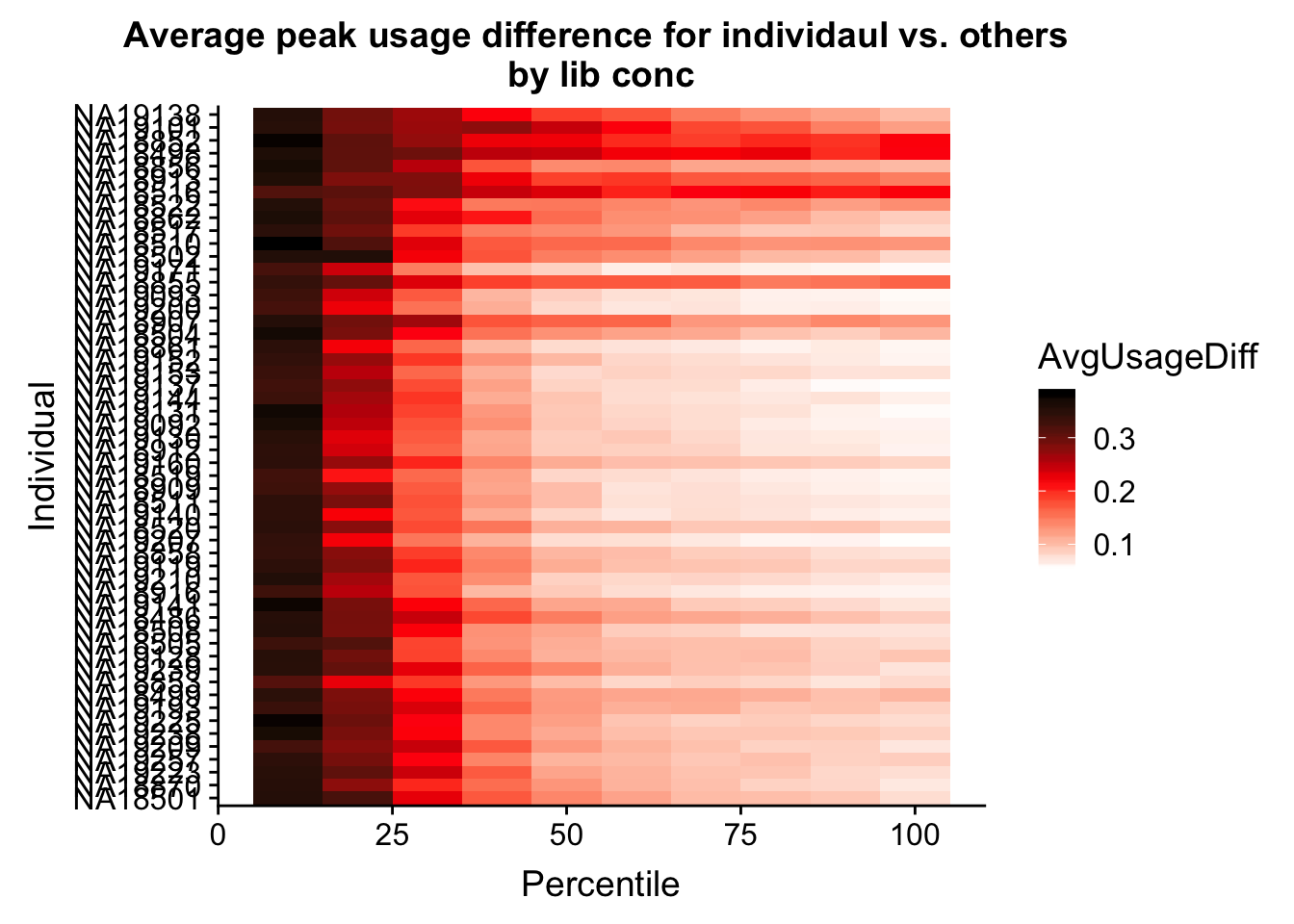 order by batch:
batch=metadataTotal %>% arrange(desc(batch))  %>% select(line) %>% mutate(sample=paste("NA" , line, sep=""))
batch=batch$sample

Percentile_df_batch=as.data.frame(Percentile) %>%   select(Percentile, batch)

#order the

Percentile_batch_melt=melt(Percentile_df_batch, id.vars=c("Percentile"))
colnames(Percentile_batch_melt)=c("Percentile", "Individual", "AvgUsageDiff")


ggplot(Percentile_batch_melt, aes(x=Percentile, y=Individual, fill=AvgUsageDiff)) + geom_tile() + labs(title="Average peak usage difference for individaul vs. others \n by batch") + scale_fill_gradientn(colours = c("white", "red", "black")) 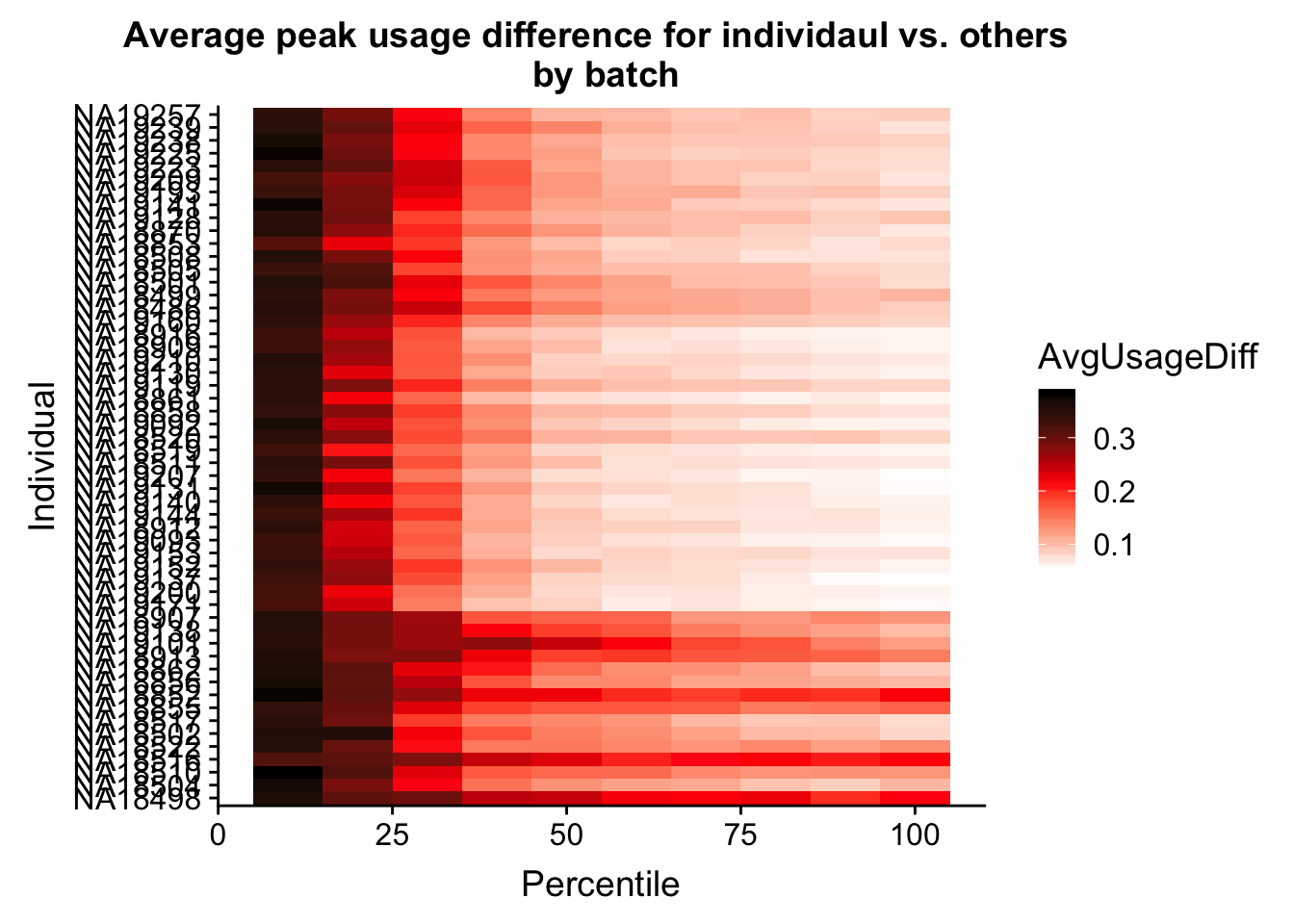
Investigate some of these meta data params:
metadataTotal$batch=as.factor(metadataTotal$batch)
reads=ggplot(metadataTotal, aes(y=reads, x=batch, fill=batch)) + geom_boxplot(position="dodge") + labs(title="Batch by read count")

conc=ggplot(metadataTotal, aes(by=batch, y=library_conc, x=batch,fill=batch)) + geom_boxplot() + labs(title="Batch by library concentration")

map=ggplot(metadataTotal, aes(by=batch, y=Mapped_noMP, x=batch,fill=batch)) + geom_boxplot() + labs(title="Batch by mapped no MP")


mapProp=ggplot(metadataTotal, aes(by=batch, y=prop_MappedwithoutMP, x=batch,fill=batch)) + geom_boxplot() + labs(title="Batch by proportion mapped no MP")


plot_grid(conc, reads, map, mapProp)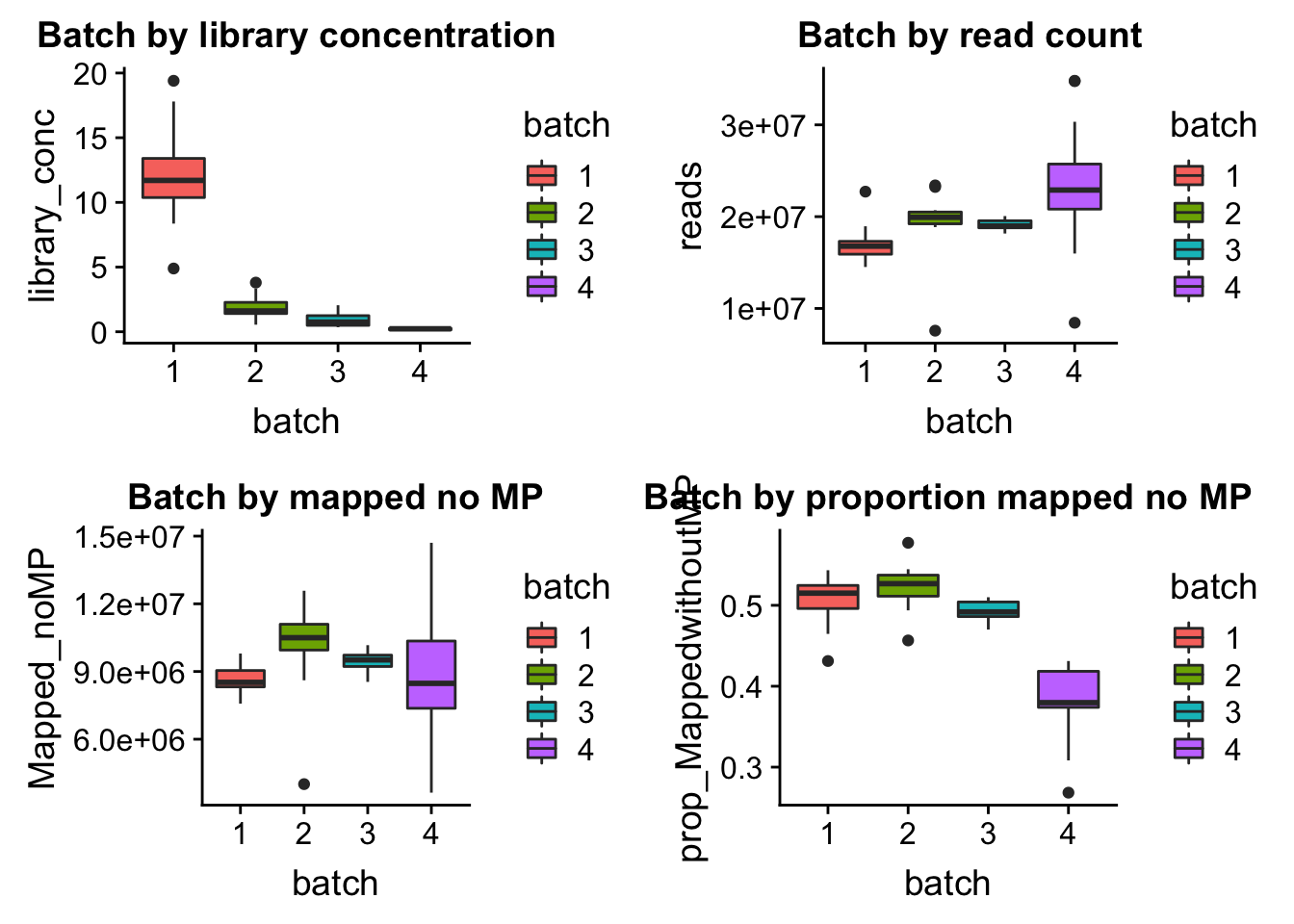
sessionInfo()R version 3.5.1 (2018-07-02)
Platform: x86_64-apple-darwin15.6.0 (64-bit)
Running under: macOS 10.14.1
Matrix products: default
BLAS: /Library/Frameworks/R.framework/Versions/3.5/Resources/lib/libRblas.0.dylib
LAPACK: /Library/Frameworks/R.framework/Versions/3.5/Resources/lib/libRlapack.dylib
locale:
[1] en_US.UTF-8/en_US.UTF-8/en_US.UTF-8/C/en_US.UTF-8/en_US.UTF-8
attached base packages:
[1] stats graphics grDevices utils datasets methods base
other attached packages:
[1] bindrcpp_0.2.2 cowplot_0.9.3 forcats_0.3.0
[4] stringr_1.4.0 dplyr_0.7.6 purrr_0.2.5
[7] readr_1.1.1 tidyr_0.8.1 tibble_1.4.2
[10] ggplot2_3.0.0 tidyverse_1.2.1 matrixStats_0.54.0
[13] reshape2_1.4.3 workflowr_1.2.0
loaded via a namespace (and not attached):
[1] Rcpp_0.12.19 cellranger_1.1.0 compiler_3.5.1 pillar_1.3.0
[5] git2r_0.24.0 plyr_1.8.4 bindr_0.1.1 tools_3.5.1
[9] digest_0.6.17 lubridate_1.7.4 jsonlite_1.6 evaluate_0.13
[13] nlme_3.1-137 gtable_0.2.0 lattice_0.20-35 pkgconfig_2.0.2
[17] rlang_0.2.2 cli_1.0.1 rstudioapi_0.9.0 yaml_2.2.0
[21] haven_1.1.2 withr_2.1.2 xml2_1.2.0 httr_1.3.1
[25] knitr_1.20 hms_0.4.2 fs_1.2.6 rprojroot_1.3-2
[29] grid_3.5.1 tidyselect_0.2.4 glue_1.3.0 R6_2.3.0
[33] readxl_1.1.0 rmarkdown_1.11 modelr_0.1.2 magrittr_1.5
[37] whisker_0.3-2 backports_1.1.2 scales_1.0.0 htmltools_0.3.6
[41] rvest_0.3.2 assertthat_0.2.0 colorspace_1.3-2 labeling_0.3
[45] stringi_1.2.4 lazyeval_0.2.1 munsell_0.5.0 broom_0.5.0
[49] crayon_1.3.4