apaQTLs by gene count percentile
Briana Mittleman
2/18/2019
Last updated: 2019-02-21
Checks: 6 0
Knit directory: threeprimeseq/analysis/
This reproducible R Markdown analysis was created with workflowr (version 1.2.0). The Report tab describes the reproducibility checks that were applied when the results were created. The Past versions tab lists the development history.
Great! Since the R Markdown file has been committed to the Git repository, you know the exact version of the code that produced these results.
Great job! The global environment was empty. Objects defined in the global environment can affect the analysis in your R Markdown file in unknown ways. For reproduciblity it’s best to always run the code in an empty environment.
The command set.seed(12345) was run prior to running the code in the R Markdown file. Setting a seed ensures that any results that rely on randomness, e.g. subsampling or permutations, are reproducible.
Great job! Recording the operating system, R version, and package versions is critical for reproducibility.
Nice! There were no cached chunks for this analysis, so you can be confident that you successfully produced the results during this run.
Great! You are using Git for version control. Tracking code development and connecting the code version to the results is critical for reproducibility. The version displayed above was the version of the Git repository at the time these results were generated.
Note that you need to be careful to ensure that all relevant files for the analysis have been committed to Git prior to generating the results (you can use wflow_publish or wflow_git_commit). workflowr only checks the R Markdown file, but you know if there are other scripts or data files that it depends on. Below is the status of the Git repository when the results were generated:
Ignored files:
    Ignored:    .DS_Store
    Ignored:    .Rhistory
    Ignored:    .Rproj.user/
    Ignored:    data/.DS_Store
    Ignored:    data/perm_QTL_trans_noMP_5percov/
    Ignored:    output/.DS_Store

Untracked files:
    Untracked:  KalistoAbundance18486.txt
    Untracked:  analysis/4suDataIGV.Rmd
    Untracked:  analysis/DirectionapaQTL.Rmd
    Untracked:  analysis/EvaleQTLs.Rmd
    Untracked:  analysis/YL_QTL_test.Rmd
    Untracked:  analysis/ncbiRefSeq_sm.sort.mRNA.bed
    Untracked:  analysis/snake.config.notes.Rmd
    Untracked:  analysis/verifyBAM.Rmd
    Untracked:  analysis/verifybam_dubs.Rmd
    Untracked:  code/PeaksToCoverPerReads.py
    Untracked:  code/strober_pc_pve_heatmap_func.R
    Untracked:  data/18486.genecov.txt
    Untracked:  data/APApeaksYL.total.inbrain.bed
    Untracked:  data/AllPeak_counts/
    Untracked:  data/ApaQTLs/
    Untracked:  data/ApaQTLs_otherPhen/
    Untracked:  data/ChromHmmOverlap/
    Untracked:  data/DistTXN2Peak_genelocAnno/
    Untracked:  data/GM12878.chromHMM.bed
    Untracked:  data/GM12878.chromHMM.txt
    Untracked:  data/LianoglouLCL/
    Untracked:  data/LocusZoom/
    Untracked:  data/LocusZoom_proc/
    Untracked:  data/MatchedSnps/
    Untracked:  data/NuclearApaQTLs.txt
    Untracked:  data/PeakCounts/
    Untracked:  data/PeakCounts_noMP_5perc/
    Untracked:  data/PeakCounts_noMP_genelocanno/
    Untracked:  data/PeakUsage/
    Untracked:  data/PeakUsage_noMP/
    Untracked:  data/PeakUsage_noMP_GeneLocAnno/
    Untracked:  data/PeaksUsed/
    Untracked:  data/PeaksUsed_noMP_5percCov/
    Untracked:  data/QTL_overlap/
    Untracked:  data/RNAkalisto/
    Untracked:  data/RefSeq_annotations/
    Untracked:  data/TotalApaQTLs.txt
    Untracked:  data/Totalpeaks_filtered_clean.bed
    Untracked:  data/UnderstandPeaksQC/
    Untracked:  data/WASP_STAT/
    Untracked:  data/YL-SP-18486-T-combined-genecov.txt
    Untracked:  data/YL-SP-18486-T_S9_R1_001-genecov.txt
    Untracked:  data/YL_QTL_test/
    Untracked:  data/apaExamp/
    Untracked:  data/apaExamp_proc/
    Untracked:  data/apaQTL_examp_noMP/
    Untracked:  data/bedgraph_peaks/
    Untracked:  data/bin200.5.T.nuccov.bed
    Untracked:  data/bin200.Anuccov.bed
    Untracked:  data/bin200.nuccov.bed
    Untracked:  data/clean_peaks/
    Untracked:  data/comb_map_stats.csv
    Untracked:  data/comb_map_stats.xlsx
    Untracked:  data/comb_map_stats_39ind.csv
    Untracked:  data/combined_reads_mapped_three_prime_seq.csv
    Untracked:  data/diff_iso_GeneLocAnno/
    Untracked:  data/diff_iso_proc/
    Untracked:  data/diff_iso_trans/
    Untracked:  data/ensemble_to_genename.txt
    Untracked:  data/example_gene_peakQuant/
    Untracked:  data/explainProtVar/
    Untracked:  data/filtPeakOppstrand_cov_noMP_GeneLocAnno_5perc/
    Untracked:  data/filtered_APApeaks_merged_allchrom_refseqTrans.closest2End.bed
    Untracked:  data/filtered_APApeaks_merged_allchrom_refseqTrans.closest2End.noties.bed
    Untracked:  data/first50lines_closest.txt
    Untracked:  data/gencov.test.csv
    Untracked:  data/gencov.test.txt
    Untracked:  data/gencov_zero.test.csv
    Untracked:  data/gencov_zero.test.txt
    Untracked:  data/gene_cov/
    Untracked:  data/joined
    Untracked:  data/leafcutter/
    Untracked:  data/merged_combined_YL-SP-threeprimeseq.bg
    Untracked:  data/molPheno_noMP/
    Untracked:  data/mol_overlap/
    Untracked:  data/mol_pheno/
    Untracked:  data/nom_QTL/
    Untracked:  data/nom_QTL_opp/
    Untracked:  data/nom_QTL_trans/
    Untracked:  data/nuc6up/
    Untracked:  data/nuc_10up/
    Untracked:  data/other_qtls/
    Untracked:  data/pQTL_otherphen/
    Untracked:  data/peakPerRefSeqGene/
    Untracked:  data/perm_QTL/
    Untracked:  data/perm_QTL_GeneLocAnno_noMP_5percov/
    Untracked:  data/perm_QTL_GeneLocAnno_noMP_5percov_3UTR/
    Untracked:  data/perm_QTL_diffWindow/
    Untracked:  data/perm_QTL_opp/
    Untracked:  data/perm_QTL_trans/
    Untracked:  data/perm_QTL_trans_filt/
    Untracked:  data/protAndAPAAndExplmRes.Rda
    Untracked:  data/protAndAPAlmRes.Rda
    Untracked:  data/protAndExpressionlmRes.Rda
    Untracked:  data/reads_mapped_three_prime_seq.csv
    Untracked:  data/smash.cov.results.bed
    Untracked:  data/smash.cov.results.csv
    Untracked:  data/smash.cov.results.txt
    Untracked:  data/smash_testregion/
    Untracked:  data/ssFC200.cov.bed
    Untracked:  data/temp.file1
    Untracked:  data/temp.file2
    Untracked:  data/temp.gencov.test.txt
    Untracked:  data/temp.gencov_zero.test.txt
    Untracked:  data/threePrimeSeqMetaData.csv
    Untracked:  data/threePrimeSeqMetaData55Ind.txt
    Untracked:  data/threePrimeSeqMetaData55Ind.xlsx
    Untracked:  data/threePrimeSeqMetaData55Ind_noDup.txt
    Untracked:  data/threePrimeSeqMetaData55Ind_noDup.xlsx
    Untracked:  data/threePrimeSeqMetaData55Ind_noDup_WASPMAP.txt
    Untracked:  data/threePrimeSeqMetaData55Ind_noDup_WASPMAP.xlsx
    Untracked:  output/deeptools_plots/
    Untracked:  output/picard/
    Untracked:  output/plots/
    Untracked:  output/qual.fig2.pdf

Unstaged changes:
    Modified:   analysis/28ind.peak.explore.Rmd
    Modified:   analysis/CompareLianoglouData.Rmd
    Modified:   analysis/NewPeakPostMP.Rmd
    Modified:   analysis/apaQTLoverlapGWAS.Rmd
    Modified:   analysis/cleanupdtseq.internalpriming.Rmd
    Modified:   analysis/coloc_apaQTLs_protQTLs.Rmd
    Modified:   analysis/dif.iso.usage.leafcutter.Rmd
    Modified:   analysis/diffIsoAnalysisNewMapping.Rmd
    Modified:   analysis/diff_iso_pipeline.Rmd
    Modified:   analysis/explainpQTLs.Rmd
    Modified:   analysis/explore.filters.Rmd
    Modified:   analysis/flash2mash.Rmd
    Modified:   analysis/mispriming_approach.Rmd
    Modified:   analysis/overlapMolQTL.Rmd
    Modified:   analysis/overlapMolQTL.opposite.Rmd
    Modified:   analysis/overlap_qtls.Rmd
    Modified:   analysis/peakOverlap_oppstrand.Rmd
    Modified:   analysis/peakQCPPlots.Rmd
    Modified:   analysis/peakQCplotsSTARprocessing.Rmd
    Modified:   analysis/pheno.leaf.comb.Rmd
    Modified:   analysis/pipeline_55Ind.Rmd
    Modified:   analysis/swarmPlots_QTLs.Rmd
    Modified:   analysis/test.max2.Rmd
    Modified:   analysis/test.smash.Rmd
    Modified:   analysis/understandPeaks.Rmd
    Modified:   code/Snakefile
Note that any generated files, e.g. HTML, png, CSS, etc., are not included in this status report because it is ok for generated content to have uncommitted changes.
These are the previous versions of the R Markdown and HTML files. If you’ve configured a remote Git repository (see ?wflow_git_remote), click on the hyperlinks in the table below to view them.
| File | Version | Author | Date | Message |
|---|---|---|---|---|
| Rmd | 9efe816 | Briana Mittleman | 2019-02-21 | add dist plots |
| html | 4e73258 | Briana Mittleman | 2019-02-19 | Build site. |
| Rmd | e0461e4 | Briana Mittleman | 2019-02-19 | add plots filtered by gene with 2 peaks |
| html | 4ea438e | Briana Mittleman | 2019-02-18 | Build site. |
| Rmd | bcb2f86 | Briana Mittleman | 2019-02-18 | add qtl by per and diff iso |
I will use this analysis to look at the number of apaQTL genes by the percentile of the counts for the gene. This may help us know if we want to sequence the libraries deeper.
library(workflowr)This is workflowr version 1.2.0
Run ?workflowr for help getting startedlibrary(tidyverse)── Attaching packages ──────────────────────────────────────────────────────────────────────────── tidyverse 1.2.1 ──✔ ggplot2 3.0.0 ✔ purrr 0.2.5
✔ tibble 1.4.2 ✔ dplyr 0.7.6
✔ tidyr 0.8.1 ✔ stringr 1.4.0
✔ readr 1.1.1 ✔ forcats 0.3.0Warning: package 'stringr' was built under R version 3.5.2── Conflicts ─────────────────────────────────────────────────────────────────────────────── tidyverse_conflicts() ──
✖ dplyr::filter() masks stats::filter()
✖ dplyr::lag() masks stats::lag()library(cowplot)
Attaching package: 'cowplot'The following object is masked from 'package:ggplot2':
ggsavelibrary(reshape2)
Attaching package: 'reshape2'The following object is masked from 'package:tidyr':
smithsQTL genes
First, upload the QTL gene.
nucQTLs=read.table("../data/ApaQTLs/NuclearapaQTLs.GeneLocAnno.noMP.5perc.10FDR.txt",stringsAsFactors = F, col.names = c("pid", "nvar", "shape1", "shape2", "dummy", "sid", "dist", "npval", "slope", "ppval", "bpval", "bh"))

nucQTLsGenes= nucQTLs%>%separate(pid, into=c("chr", "start", "end", "id"), sep=":") %>% separate(id, into=c("gene", "strand", "peak"), sep="_") %>% select(gene) %>% unique()


totQTLs=read.table("../data/ApaQTLs/TotalapaQTLs.GeneLocAnno.noMP.5perc.10FDR.txt",stringsAsFactors = F, col.names = c("pid", "nvar", "shape1", "shape2", "dummy", "sid", "dist", "npval", "slope", "ppval", "bpval", "bh"))

totQTLsGenes= totQTLs%>%separate(pid, into=c("chr", "start", "end", "id"), sep=":") %>% separate(id, into=c("gene", "strand", "peak"), sep="_") %>% select(gene) %>% unique()
How many of the genes overlap:
QTLgene_both=totQTLsGenes %>% inner_join(nucQTLsGenes, by="gene")
nrow(QTLgene_both)
[1] 141This means 141 genes have a QTL for both. It does not tell me if the QTL is the same.
Gene Counts
I can get this from the prefiltered peak counts. /project2/gilad/briana/threeprimeseq/data/filtPeakOppstrand_cov_noMP_GeneLocAnno/filtered_APApeaks_merged_allchrom_refseqGenes.GeneLocAnno_NoMP_sm_quant.Total.fixed.fc
/project2/gilad/briana/threeprimeseq/data/filtPeakOppstrand_cov_noMP_GeneLocAnno/filtered_APApeaks_merged_allchrom_refseqGenes.GeneLocAnno_NoMP_sm_quant.Nuclear.fixed.fc
I can pull these files in, group them by gene and get summaries.
Total
totPeakCounts=read.table("../data/AllPeak_counts/filtered_APApeaks_merged_allchrom_refseqGenes.GeneLocAnno_NoMP_sm_quant.Total.fixed.fc", header = T, stringsAsFactors = F) %>% select(-Chr, -Start, -End, -Strand, -Length) %>% separate(Geneid, into=c("peak", "chr", "start", "end", "strand", "gene"), sep=":") %>% select(-peak, -chr,-start, -end, -strand, -gene)
totPeakCountsGene=read.table("../data/AllPeak_counts/filtered_APApeaks_merged_allchrom_refseqGenes.GeneLocAnno_NoMP_sm_quant.Total.fixed.fc", header = T, stringsAsFactors = F) %>% select(-Chr, -Start, -End, -Strand, -Length) %>% separate(Geneid, into=c("peak", "chr", "start", "end", "strand", "gene"), sep=":") %>% select(gene)
#sum across ind.
totPeakCounts_Sum=rowSums(totPeakCounts)
totPeakCountsGeneSum=as.data.frame(cbind(totPeakCountsGene,totPeakCounts_Sum)) %>% group_by(gene) %>% summarise(TotalCount=sum(totPeakCounts_Sum)) %>% mutate(Percentile = percent_rank(TotalCount))
Subset by percetile:
totalCount_10= totPeakCountsGeneSum %>% filter(Percentile<.1)
totalCount_20= totPeakCountsGeneSum %>% filter(Percentile<.2, Percentile>.1)
totalCount_30= totPeakCountsGeneSum %>% filter(Percentile<.3, Percentile>.2)
totalCount_40= totPeakCountsGeneSum %>% filter(Percentile<.4, Percentile>.3)
totalCount_50= totPeakCountsGeneSum %>% filter(Percentile<.5, Percentile>.4)
totalCount_60= totPeakCountsGeneSum %>% filter(Percentile<.6, Percentile>.5)
totalCount_70= totPeakCountsGeneSum %>% filter(Percentile<.7, Percentile>.6)
totalCount_80= totPeakCountsGeneSum %>% filter(Percentile<.8, Percentile>.7)
totalCount_90= totPeakCountsGeneSum %>% filter(Percentile<.9, Percentile>.8)
totalCount_100= totPeakCountsGeneSum %>% filter(Percentile<1, Percentile>.9)
Nuclear
nucPeakCounts=read.table("../data/AllPeak_counts/filtered_APApeaks_merged_allchrom_refseqGenes.GeneLocAnno_NoMP_sm_quant.Nuclear.fixed.fc", header = T, stringsAsFactors = F) %>% select(-Chr, -Start, -End, -Strand, -Length) %>% separate(Geneid, into=c("peak", "chr", "start", "end", "strand", "gene"), sep=":") %>% select(-peak, -chr,-start, -end, -strand, -gene)
nucPeakCountsGene=read.table("../data/AllPeak_counts/filtered_APApeaks_merged_allchrom_refseqGenes.GeneLocAnno_NoMP_sm_quant.Nuclear.fixed.fc", header = T, stringsAsFactors = F) %>% select(-Chr, -Start, -End, -Strand, -Length) %>% separate(Geneid, into=c("peak", "chr", "start", "end", "strand", "gene"), sep=":") %>% select(gene)
#sum across ind.
nucPeakCounts_Sum=rowSums(nucPeakCounts)
nucPeakCountsGeneSum=as.data.frame(cbind(nucPeakCountsGene,nucPeakCounts_Sum)) %>% group_by(gene) %>% summarise(NuclearCount=sum(nucPeakCounts_Sum)) %>% mutate(Percentile = percent_rank(NuclearCount))
nuclearCount_10= nucPeakCountsGeneSum %>% filter(Percentile<.1)
nuclearCount_20= nucPeakCountsGeneSum %>% filter(Percentile<.2, Percentile>.1)
nuclearCount_30= nucPeakCountsGeneSum %>% filter(Percentile<.3, Percentile>.2)
nuclearCount_40= nucPeakCountsGeneSum %>% filter(Percentile<.4, Percentile>.3)
nuclearCount_50= nucPeakCountsGeneSum %>% filter(Percentile<.5, Percentile>.4)
nuclearCount_60= nucPeakCountsGeneSum %>% filter(Percentile<.6, Percentile>.5)
nuclearCount_70= nucPeakCountsGeneSum %>% filter(Percentile<.7, Percentile>.6)
nuclearCount_80= nucPeakCountsGeneSum %>% filter(Percentile<.8, Percentile>.7)
nuclearCount_90= nucPeakCountsGeneSum %>% filter(Percentile<.9, Percentile>.8)
nuclearCount_100= nucPeakCountsGeneSum %>% filter(Percentile<1, Percentile>.9)QTL genes
I can get the percentile for each QTL gene.
totQTLGene_Perc= totQTLsGenes %>% inner_join(totPeakCountsGeneSum, by="gene") %>% mutate(roundPerc=round(Percentile, digits=1)) %>% group_by(roundPerc) %>% summarise(Ngenes=n())
nucQTLGene_Perc= nucQTLsGenes %>% inner_join(nucPeakCountsGeneSum, by="gene")%>% mutate(roundPerc=round(Percentile, digits=1)) %>% group_by(roundPerc) %>% summarise(Ngenes=n())

bothPerc=totQTLGene_Perc %>% full_join(nucQTLGene_Perc,  by = c("roundPerc"))
bothPerc$Ngenes.x= bothPerc$Ngenes.x %>% replace_na(0)
colnames(bothPerc)= c("Percentile", "Total", "Nuclear")


bothPerc_melt= melt(bothPerc, id.vars = "Percentile")
colnames(bothPerc_melt) =c("Percentile", "Fraction", "Genes")
Plot:
ggplot(bothPerc_melt, aes(x=Percentile, y= Genes, by=Fraction, fill=Fraction)) + geom_bar(stat="identity", position = "dodge") + theme(axis.text.y = element_text(size=12),axis.title.y=element_text(size=10,face="bold"), axis.title.x=element_text(size=12,face="bold"))+ scale_fill_manual(values=c("darkviolet","deepskyblue3")) 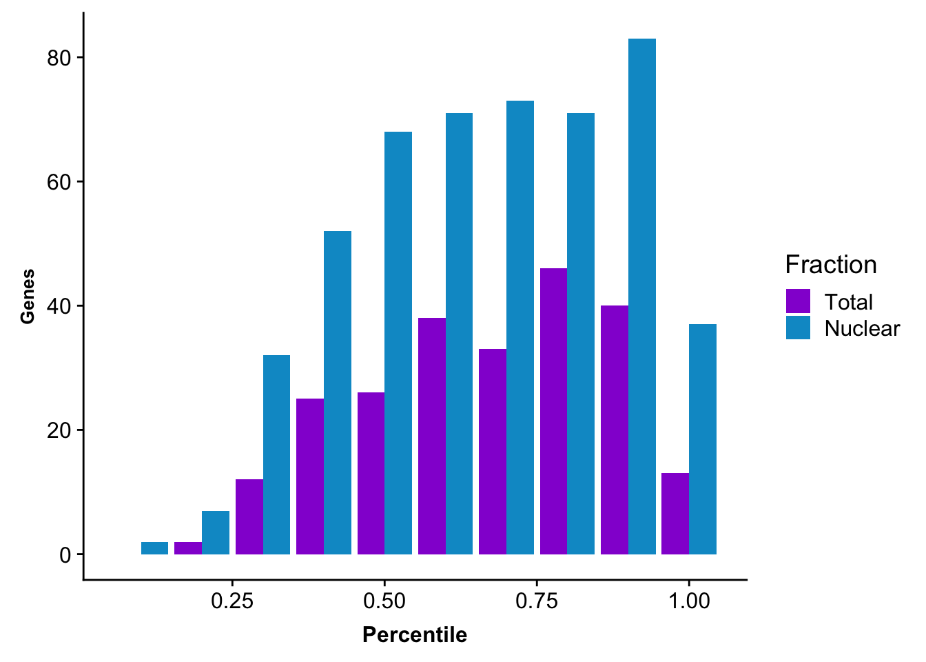
| Version | Author | Date |
|---|---|---|
| 4ea438e | Briana Mittleman | 2019-02-18 |
To make is a percente of genes in the category I will divide each number of genes category by the number of total QTL genes. For total this is 291 and for nuclear it is 496
totQTLGene_Perc_prop= totQTLsGenes %>% inner_join(totPeakCountsGeneSum, by="gene") %>% mutate(roundPerc=round(Percentile, digits=1)) %>% group_by(roundPerc) %>% summarise(Ngenes=n()) %>% mutate(PercGenes=Ngenes/291)
nucQTLGene_Perc_prop= nucQTLsGenes %>% inner_join(nucPeakCountsGeneSum, by="gene")%>% mutate(roundPerc=round(Percentile, digits=1)) %>% group_by(roundPerc) %>% summarise(Ngenes=n()) %>%mutate(PercGenes=Ngenes/496)


bothPercProp=totQTLGene_Perc_prop %>% full_join(nucQTLGene_Perc_prop,  by = c("roundPerc")) %>% select(roundPerc, starts_with("perc"))
bothPercProp$PercGenes.x= bothPercProp$PercGenes.x %>% replace_na(0)
colnames(bothPercProp)= c("Percentile", "Total", "Nuclear")


bothPercPrp_melt= melt(bothPercProp, id.vars = "Percentile")
colnames(bothPercPrp_melt) =c("Percentile", "Fraction", "GenesProp")
QTLSbyCountPerc=ggplot(bothPercPrp_melt, aes(x=Percentile, y=GenesProp, fill=Fraction)) +geom_bar(stat="identity", position = "dodge")+labs(title="Proportion of QTL genes by Read count percentile",y="Proportion of QTLs", x="Read Cound percentile") + theme(axis.text.y = element_text(size=12),axis.title.y=element_text(size=10,face="bold"), axis.title.x=element_text(size=12,face="bold"))+ scale_fill_manual(values=c("darkviolet","deepskyblue3")) + facet_grid(~Fraction)
QTLSbyCountPerc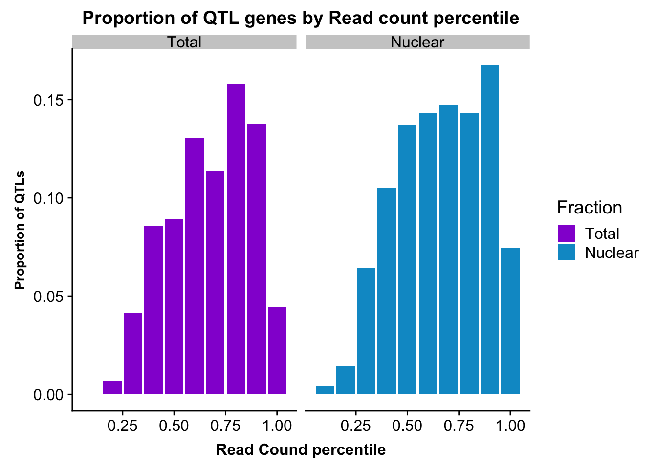
| Version | Author | Date |
|---|---|---|
| 4ea438e | Briana Mittleman | 2019-02-18 |
ggsave(QTLSbyCountPerc, file="../output/plots/QTLSbyCountPerc.png")Saving 7 x 5 in imageFilter to only look at genes with at least 2 peaks and build the percentiles off these. To do this I will filter the unfiltered peak counts by genes with two peaks in the 5% peaks used in the QTL analysis.
Pull in filtered peaks:
Peaks=read.table("../data/PeakUsage_noMP_GeneLocAnno/Filtered_APApeaks_merged_allchrom_noMP.sort.named.noCHR_geneLocParsed.5percCov.bed", stringsAsFactors = F, col.names = c("chr", 'start', 'end', 'id', 'score', 'strand'))
Genes2Peaks= Peaks %>% separate(id, into=c("gene", "peak"), sep=":") %>% group_by(gene) %>% summarise(nPeak=n()) %>% filter(nPeak>=2) %>% select(gene)
Now filter the total and nuclear peaks that are in these genes before making the percentile plots.
Total
totPeakCounts_FiltGene=read.table("../data/AllPeak_counts/filtered_APApeaks_merged_allchrom_refseqGenes.GeneLocAnno_NoMP_sm_quant.Total.fixed.fc", header = T, stringsAsFactors = F) %>% select(-Chr, -Start, -End, -Strand, -Length) %>% separate(Geneid, into=c("peak", "chr", "start", "end", "strand", "gene"), sep=":") %>% semi_join(Genes2Peaks, by="gene")%>% select(-peak, -chr,-start, -end, -strand, -gene)

totPeakCountsFiltGene=read.table("../data/AllPeak_counts/filtered_APApeaks_merged_allchrom_refseqGenes.GeneLocAnno_NoMP_sm_quant.Total.fixed.fc", header = T, stringsAsFactors = F) %>% select(-Chr, -Start, -End, -Strand, -Length) %>% separate(Geneid, into=c("peak", "chr", "start", "end", "strand", "gene"), sep=":") %>% semi_join(Genes2Peaks, by="gene") %>% select(gene)
#sum across ind.
totPeakCounts_FiltSum=rowSums(totPeakCounts_FiltGene)
totPeakCountsFiltGeneSum=as.data.frame(cbind(totPeakCountsFiltGene,totPeakCounts_FiltSum)) %>% group_by(gene) %>% summarise(TotalCount=sum(totPeakCounts_FiltSum)) %>% mutate(Percentile = percent_rank(TotalCount))
Nuclear
nucPeakCounts_FiltGene=read.table("../data/AllPeak_counts/filtered_APApeaks_merged_allchrom_refseqGenes.GeneLocAnno_NoMP_sm_quant.Nuclear.fixed.fc", header = T, stringsAsFactors = F) %>% select(-Chr, -Start, -End, -Strand, -Length) %>% separate(Geneid, into=c("peak", "chr", "start", "end", "strand", "gene"), sep=":") %>% semi_join(Genes2Peaks, by="gene")%>% select(-peak, -chr,-start, -end, -strand, -gene)

nucPeakCountsFiltGene=read.table("../data/AllPeak_counts/filtered_APApeaks_merged_allchrom_refseqGenes.GeneLocAnno_NoMP_sm_quant.Nuclear.fixed.fc", header = T, stringsAsFactors = F) %>% select(-Chr, -Start, -End, -Strand, -Length) %>% separate(Geneid, into=c("peak", "chr", "start", "end", "strand", "gene"), sep=":") %>% semi_join(Genes2Peaks, by="gene") %>% select(gene)
#sum across ind.
nucPeakCounts_FiltSum=rowSums(nucPeakCounts_FiltGene)
nucPeakCountsFiltGeneSum=as.data.frame(cbind(nucPeakCountsFiltGene,nucPeakCounts_FiltSum)) %>% group_by(gene) %>% summarise(NuclearCount=sum(nucPeakCounts_FiltSum)) %>% mutate(Percentile = percent_rank(NuclearCount))
I can get the percentile for each QTL gene.
totQTLFiltGene_Perc= totQTLsGenes %>% inner_join(totPeakCountsFiltGeneSum, by="gene") %>% mutate(roundPerc=round(Percentile, digits=1)) %>% group_by(roundPerc) %>% summarise(Ngenes=n())
nucQTLFiltGene_Perc= nucQTLsGenes %>% inner_join(nucPeakCountsFiltGeneSum, by="gene")%>% mutate(roundPerc=round(Percentile, digits=1)) %>% group_by(roundPerc) %>% summarise(Ngenes=n())

bothPerc_filt=totQTLFiltGene_Perc %>% full_join(nucQTLFiltGene_Perc,  by = c("roundPerc"))
bothPerc_filt$Ngenes.x= bothPerc_filt$Ngenes.x %>% replace_na(0)
colnames(bothPerc_filt)= c("Percentile", "Total", "Nuclear")


bothPercfilt_melt= melt(bothPerc_filt, id.vars = "Percentile")
colnames(bothPercfilt_melt) =c("Percentile", "Fraction", "Genes")
Plot:
ggplot(bothPercfilt_melt, aes(x=Percentile, y= Genes, by=Fraction, fill=Fraction)) + geom_bar(stat="identity", position = "dodge") + theme(axis.text.y = element_text(size=12),axis.title.y=element_text(size=10,face="bold"), axis.title.x=element_text(size=12,face="bold"))+ scale_fill_manual(values=c("darkviolet","deepskyblue3")) 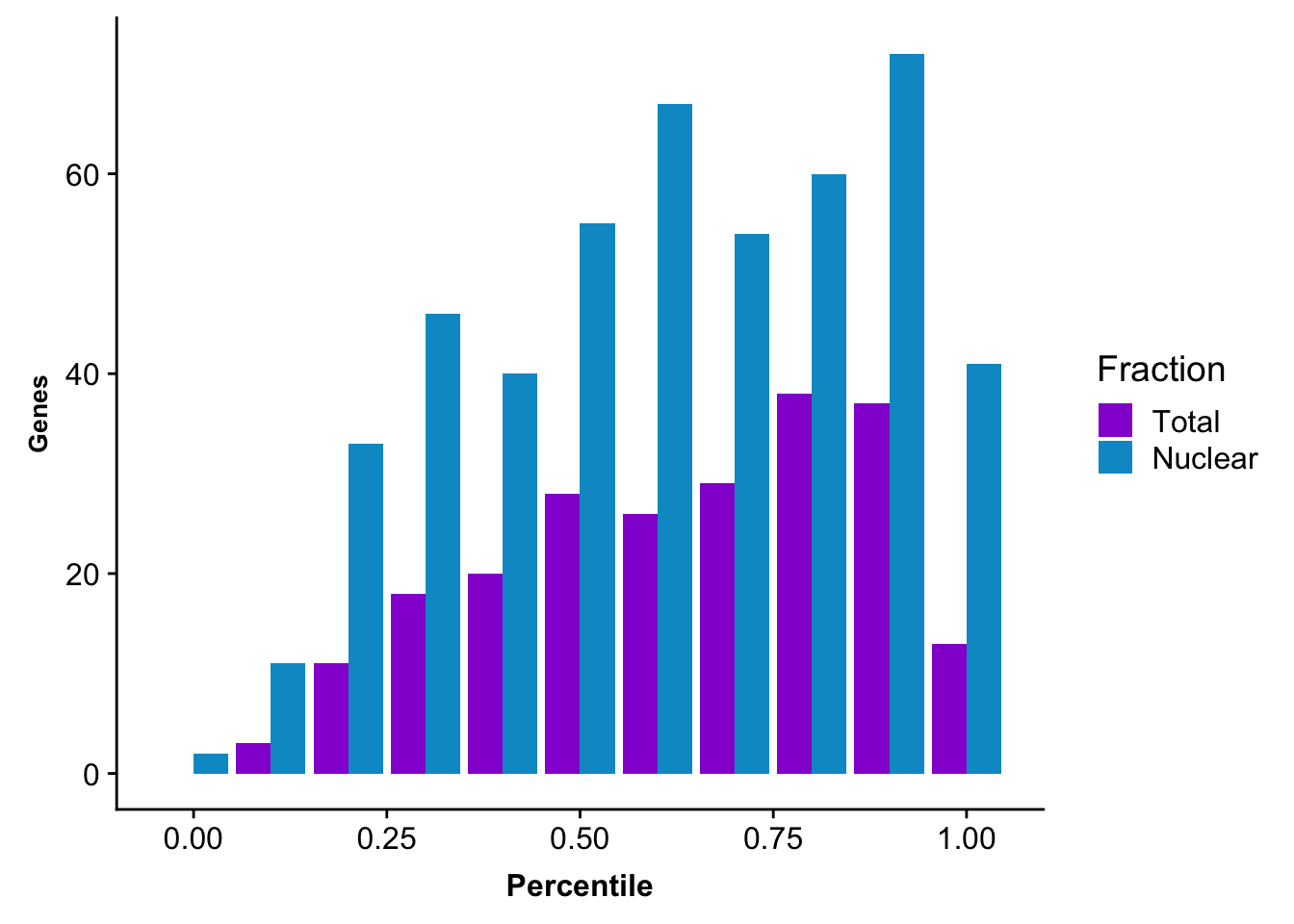
| Version | Author | Date |
|---|---|---|
| 4e73258 | Briana Mittleman | 2019-02-19 |
Do it by percent
totQTLFiltGene_Perc_prop= totQTLsGenes %>% inner_join(totPeakCountsFiltGeneSum, by="gene") %>% mutate(roundPerc=round(Percentile, digits=1)) %>% group_by(roundPerc) %>% summarise(Ngenes=n()) %>% mutate(PercGenes=Ngenes/291)
nucQTLFiltGene_Perc_prop= nucQTLsGenes %>% inner_join(nucPeakCountsFiltGeneSum, by="gene")%>% mutate(roundPerc=round(Percentile, digits=1)) %>% group_by(roundPerc) %>% summarise(Ngenes=n()) %>%mutate(PercGenes=Ngenes/496)


bothPercFiltProp=totQTLFiltGene_Perc_prop %>% full_join(nucQTLFiltGene_Perc_prop,  by = c("roundPerc")) %>% select(roundPerc, starts_with("perc"))
bothPercFiltProp$PercGenes.x= bothPercFiltProp$PercGenes.x %>% replace_na(0)
colnames(bothPercFiltProp)= c("Percentile", "Total", "Nuclear")


bothPercPrpFilt_melt= melt(bothPercFiltProp, id.vars = "Percentile")
colnames(bothPercPrpFilt_melt) =c("Percentile", "Fraction", "GenesProp")
QTLSbyCountPerc_filt=ggplot(bothPercPrpFilt_melt, aes(x=Percentile, y=GenesProp, fill=Fraction)) +geom_bar(stat="identity", position = "dodge")+labs(title="Proportion of QTL genes by Read count percentile\n Genes with 2 peaks in QTL analysis",y="Proportion of QTLs", x="Read Cound percentile") + theme(axis.text.y = element_text(size=12),axis.title.y=element_text(size=10,face="bold"), axis.title.x=element_text(size=12,face="bold"))+ scale_fill_manual(values=c("darkviolet","deepskyblue3")) + facet_grid(~Fraction)
QTLSbyCountPerc_filt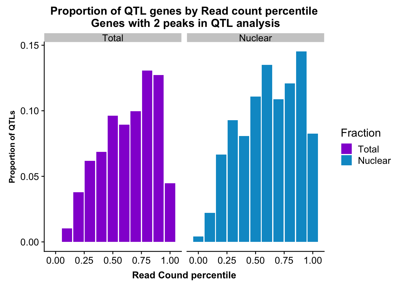
| Version | Author | Date |
|---|---|---|
| 4e73258 | Briana Mittleman | 2019-02-19 |
ggsave(QTLSbyCountPerc_filt, file="../output/plots/QTLSbyCountPerc_Genes2Peaks.png")Saving 7 x 5 in imageDont round: look at distibution:
totperc=totQTLsGenes %>% inner_join(totPeakCountsFiltGeneSum, by="gene")

totbyexp=ggplot(totperc, aes(x=Percentile)) + geom_density(fill="darkviolet") + labs(x="Count Percentile" ,title="Total Apa QTLs by Count Percentile")
nucperc=nucQTLsGenes %>% inner_join(nucPeakCountsFiltGeneSum, by="gene")
nucbyexp=ggplot(nucperc, aes(x=Percentile)) + geom_density(fill="deepskyblue3") + labs(x="Count Percentile" ,title="Nuclear Apa QTLs by Count Percentile") bothQTLbyExp=plot_grid(totbyexp,nucbyexp)
bothQTLbyExp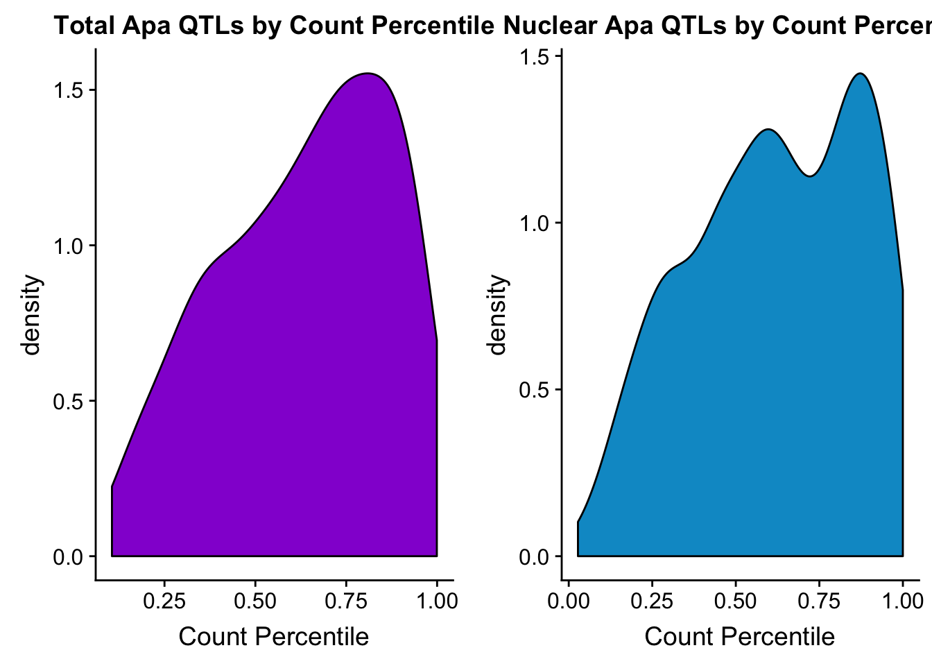
ggsave(bothQTLbyExp, file="../output/plots/BothQTLSbyCountPerc_Genes2Peaks_density.png")Saving 7 x 5 in image
sessionInfo()R version 3.5.1 (2018-07-02)
Platform: x86_64-apple-darwin15.6.0 (64-bit)
Running under: macOS 10.14.1
Matrix products: default
BLAS: /Library/Frameworks/R.framework/Versions/3.5/Resources/lib/libRblas.0.dylib
LAPACK: /Library/Frameworks/R.framework/Versions/3.5/Resources/lib/libRlapack.dylib
locale:
[1] en_US.UTF-8/en_US.UTF-8/en_US.UTF-8/C/en_US.UTF-8/en_US.UTF-8
attached base packages:
[1] stats graphics grDevices utils datasets methods base
other attached packages:
[1] bindrcpp_0.2.2 reshape2_1.4.3 cowplot_0.9.3 forcats_0.3.0
[5] stringr_1.4.0 dplyr_0.7.6 purrr_0.2.5 readr_1.1.1
[9] tidyr_0.8.1 tibble_1.4.2 ggplot2_3.0.0 tidyverse_1.2.1
[13] workflowr_1.2.0
loaded via a namespace (and not attached):
[1] tidyselect_0.2.4 haven_1.1.2 lattice_0.20-35 colorspace_1.3-2
[5] htmltools_0.3.6 yaml_2.2.0 rlang_0.2.2 pillar_1.3.0
[9] glue_1.3.0 withr_2.1.2 modelr_0.1.2 readxl_1.1.0
[13] bindr_0.1.1 plyr_1.8.4 munsell_0.5.0 gtable_0.2.0
[17] cellranger_1.1.0 rvest_0.3.2 evaluate_0.13 labeling_0.3
[21] knitr_1.20 broom_0.5.0 Rcpp_0.12.19 scales_1.0.0
[25] backports_1.1.2 jsonlite_1.6 fs_1.2.6 hms_0.4.2
[29] digest_0.6.17 stringi_1.2.4 grid_3.5.1 rprojroot_1.3-2
[33] cli_1.0.1 tools_3.5.1 magrittr_1.5 lazyeval_0.2.1
[37] crayon_1.3.4 whisker_0.3-2 pkgconfig_2.0.2 xml2_1.2.0
[41] lubridate_1.7.4 assertthat_0.2.0 rmarkdown_1.11 httr_1.3.1
[45] rstudioapi_0.9.0 R6_2.3.0 nlme_3.1-137 git2r_0.24.0
[49] compiler_3.5.1