Characterize Total ApaQTLs
Briana Mittleman
10/11/2018
Last updated: 2019-02-15
Checks: 6 0
Knit directory: threeprimeseq/analysis/
This reproducible R Markdown analysis was created with workflowr (version 1.2.0). The Report tab describes the reproducibility checks that were applied when the results were created. The Past versions tab lists the development history.
Great! Since the R Markdown file has been committed to the Git repository, you know the exact version of the code that produced these results.
Great job! The global environment was empty. Objects defined in the global environment can affect the analysis in your R Markdown file in unknown ways. For reproduciblity it’s best to always run the code in an empty environment.
The command set.seed(12345) was run prior to running the code in the R Markdown file. Setting a seed ensures that any results that rely on randomness, e.g. subsampling or permutations, are reproducible.
Great job! Recording the operating system, R version, and package versions is critical for reproducibility.
Nice! There were no cached chunks for this analysis, so you can be confident that you successfully produced the results during this run.
Great! You are using Git for version control. Tracking code development and connecting the code version to the results is critical for reproducibility. The version displayed above was the version of the Git repository at the time these results were generated.
Note that you need to be careful to ensure that all relevant files for the analysis have been committed to Git prior to generating the results (you can use wflow_publish or wflow_git_commit). workflowr only checks the R Markdown file, but you know if there are other scripts or data files that it depends on. Below is the status of the Git repository when the results were generated:
Ignored files:
    Ignored:    .DS_Store
    Ignored:    .Rhistory
    Ignored:    .Rproj.user/
    Ignored:    data/.DS_Store
    Ignored:    data/perm_QTL_trans_noMP_5percov/
    Ignored:    output/.DS_Store

Untracked files:
    Untracked:  KalistoAbundance18486.txt
    Untracked:  analysis/4suDataIGV.Rmd
    Untracked:  analysis/DirectionapaQTL.Rmd
    Untracked:  analysis/EvaleQTLs.Rmd
    Untracked:  analysis/YL_QTL_test.Rmd
    Untracked:  analysis/ncbiRefSeq_sm.sort.mRNA.bed
    Untracked:  analysis/snake.config.notes.Rmd
    Untracked:  analysis/verifyBAM.Rmd
    Untracked:  analysis/verifybam_dubs.Rmd
    Untracked:  code/PeaksToCoverPerReads.py
    Untracked:  code/strober_pc_pve_heatmap_func.R
    Untracked:  data/18486.genecov.txt
    Untracked:  data/APApeaksYL.total.inbrain.bed
    Untracked:  data/ApaQTLs/
    Untracked:  data/ChromHmmOverlap/
    Untracked:  data/DistTXN2Peak_genelocAnno/
    Untracked:  data/GM12878.chromHMM.bed
    Untracked:  data/GM12878.chromHMM.txt
    Untracked:  data/LianoglouLCL/
    Untracked:  data/LocusZoom/
    Untracked:  data/NuclearApaQTLs.txt
    Untracked:  data/PeakCounts/
    Untracked:  data/PeakCounts_noMP_5perc/
    Untracked:  data/PeakCounts_noMP_genelocanno/
    Untracked:  data/PeakUsage/
    Untracked:  data/PeakUsage_noMP/
    Untracked:  data/PeakUsage_noMP_GeneLocAnno/
    Untracked:  data/PeaksUsed/
    Untracked:  data/PeaksUsed_noMP_5percCov/
    Untracked:  data/RNAkalisto/
    Untracked:  data/RefSeq_annotations/
    Untracked:  data/TotalApaQTLs.txt
    Untracked:  data/Totalpeaks_filtered_clean.bed
    Untracked:  data/UnderstandPeaksQC/
    Untracked:  data/WASP_STAT/
    Untracked:  data/YL-SP-18486-T-combined-genecov.txt
    Untracked:  data/YL-SP-18486-T_S9_R1_001-genecov.txt
    Untracked:  data/YL_QTL_test/
    Untracked:  data/apaExamp/
    Untracked:  data/apaQTL_examp_noMP/
    Untracked:  data/bedgraph_peaks/
    Untracked:  data/bin200.5.T.nuccov.bed
    Untracked:  data/bin200.Anuccov.bed
    Untracked:  data/bin200.nuccov.bed
    Untracked:  data/clean_peaks/
    Untracked:  data/comb_map_stats.csv
    Untracked:  data/comb_map_stats.xlsx
    Untracked:  data/comb_map_stats_39ind.csv
    Untracked:  data/combined_reads_mapped_three_prime_seq.csv
    Untracked:  data/diff_iso_GeneLocAnno/
    Untracked:  data/diff_iso_proc/
    Untracked:  data/diff_iso_trans/
    Untracked:  data/ensemble_to_genename.txt
    Untracked:  data/example_gene_peakQuant/
    Untracked:  data/explainProtVar/
    Untracked:  data/filtPeakOppstrand_cov_noMP_GeneLocAnno_5perc/
    Untracked:  data/filtered_APApeaks_merged_allchrom_refseqTrans.closest2End.bed
    Untracked:  data/filtered_APApeaks_merged_allchrom_refseqTrans.closest2End.noties.bed
    Untracked:  data/first50lines_closest.txt
    Untracked:  data/gencov.test.csv
    Untracked:  data/gencov.test.txt
    Untracked:  data/gencov_zero.test.csv
    Untracked:  data/gencov_zero.test.txt
    Untracked:  data/gene_cov/
    Untracked:  data/joined
    Untracked:  data/leafcutter/
    Untracked:  data/merged_combined_YL-SP-threeprimeseq.bg
    Untracked:  data/molPheno_noMP/
    Untracked:  data/mol_overlap/
    Untracked:  data/mol_pheno/
    Untracked:  data/nom_QTL/
    Untracked:  data/nom_QTL_opp/
    Untracked:  data/nom_QTL_trans/
    Untracked:  data/nuc6up/
    Untracked:  data/nuc_10up/
    Untracked:  data/other_qtls/
    Untracked:  data/pQTL_otherphen/
    Untracked:  data/peakPerRefSeqGene/
    Untracked:  data/perm_QTL/
    Untracked:  data/perm_QTL_GeneLocAnno_noMP_5percov/
    Untracked:  data/perm_QTL_GeneLocAnno_noMP_5percov_3UTR/
    Untracked:  data/perm_QTL_opp/
    Untracked:  data/perm_QTL_trans/
    Untracked:  data/perm_QTL_trans_filt/
    Untracked:  data/protAndAPAAndExplmRes.Rda
    Untracked:  data/protAndAPAlmRes.Rda
    Untracked:  data/protAndExpressionlmRes.Rda
    Untracked:  data/reads_mapped_three_prime_seq.csv
    Untracked:  data/smash.cov.results.bed
    Untracked:  data/smash.cov.results.csv
    Untracked:  data/smash.cov.results.txt
    Untracked:  data/smash_testregion/
    Untracked:  data/ssFC200.cov.bed
    Untracked:  data/temp.file1
    Untracked:  data/temp.file2
    Untracked:  data/temp.gencov.test.txt
    Untracked:  data/temp.gencov_zero.test.txt
    Untracked:  data/threePrimeSeqMetaData.csv
    Untracked:  data/threePrimeSeqMetaData55Ind.txt
    Untracked:  data/threePrimeSeqMetaData55Ind.xlsx
    Untracked:  data/threePrimeSeqMetaData55Ind_noDup.txt
    Untracked:  data/threePrimeSeqMetaData55Ind_noDup.xlsx
    Untracked:  data/threePrimeSeqMetaData55Ind_noDup_WASPMAP.txt
    Untracked:  data/threePrimeSeqMetaData55Ind_noDup_WASPMAP.xlsx
    Untracked:  output/picard/
    Untracked:  output/plots/
    Untracked:  output/qual.fig2.pdf

Unstaged changes:
    Modified:   analysis/28ind.peak.explore.Rmd
    Modified:   analysis/CompareLianoglouData.Rmd
    Modified:   analysis/NewPeakPostMP.Rmd
    Modified:   analysis/apaQTLoverlapGWAS.Rmd
    Modified:   analysis/cleanupdtseq.internalpriming.Rmd
    Modified:   analysis/coloc_apaQTLs_protQTLs.Rmd
    Modified:   analysis/dif.iso.usage.leafcutter.Rmd
    Modified:   analysis/diff_iso_pipeline.Rmd
    Modified:   analysis/explainpQTLs.Rmd
    Modified:   analysis/explore.filters.Rmd
    Modified:   analysis/flash2mash.Rmd
    Modified:   analysis/mispriming_approach.Rmd
    Modified:   analysis/overlapMolQTL.Rmd
    Modified:   analysis/overlapMolQTL.opposite.Rmd
    Modified:   analysis/overlap_qtls.Rmd
    Modified:   analysis/peakOverlap_oppstrand.Rmd
    Modified:   analysis/peakQCPPlots.Rmd
    Modified:   analysis/pheno.leaf.comb.Rmd
    Modified:   analysis/pipeline_55Ind.Rmd
    Modified:   analysis/swarmPlots_QTLs.Rmd
    Modified:   analysis/test.max2.Rmd
    Modified:   analysis/test.smash.Rmd
    Modified:   analysis/understandPeaks.Rmd
    Modified:   code/Snakefile
Note that any generated files, e.g. HTML, png, CSS, etc., are not included in this status report because it is ok for generated content to have uncommitted changes.
These are the previous versions of the R Markdown and HTML files. If you’ve configured a remote Git repository (see ?wflow_git_remote), click on the hyperlinks in the table below to view them.
| File | Version | Author | Date | Message |
|---|---|---|---|---|
| html | de24d7d | Briana Mittleman | 2019-01-15 | Build site. |
| Rmd | 57fbf88 | Briana Mittleman | 2019-01-15 | update dist to peak plots |
| html | a5b4cf6 | Briana Mittleman | 2018-10-29 | Build site. |
| Rmd | afb0ce9 | Briana Mittleman | 2018-10-29 | change plot colors |
| html | 96cfdcd | Briana Mittleman | 2018-10-24 | Build site. |
| Rmd | 00b1020 | Briana Mittleman | 2018-10-24 | naive enrichment |
| html | cb92826 | Briana Mittleman | 2018-10-23 | Build site. |
| Rmd | 59d9b4a | Briana Mittleman | 2018-10-23 | add chromHMM enrichment Total |
| html | 12db557 | Briana Mittleman | 2018-10-23 | Build site. |
| html | d7106c9 | Briana Mittleman | 2018-10-15 | Build site. |
| Rmd | fb433ec | Briana Mittleman | 2018-10-15 | make bed with sig snps |
| html | 2f4b083 | Briana Mittleman | 2018-10-12 | Build site. |
| Rmd | 467b7a2 | Briana Mittleman | 2018-10-12 | process HMM annoatiotn |
| html | bb6c0de | Briana Mittleman | 2018-10-12 | Build site. |
| Rmd | d889cd4 | Briana Mittleman | 2018-10-12 | add QTL sig by peak score plot |
| html | f771110 | Briana Mittleman | 2018-10-12 | Build site. |
| Rmd | 477c3f2 | Briana Mittleman | 2018-10-12 | add mean exp and var plots |
| html | eb02fbc | Briana Mittleman | 2018-10-11 | Build site. |
| Rmd | f819c8e | Briana Mittleman | 2018-10-11 | add distance metric analsis total apaQTL |
This analysis will be used to characterize the total ApaQTLs. I will run the analysis on the total APAqtls in this analysis and will then run a similar analysis on the nuclear APAqtls in another analysis. I would like to study:
- Distance metrics:
- distance from snp to TSS of gene
- Distance from snp to peak
- distance from snp to TSS of gene
- Expression metrics:
- expression of genes with significant QTLs vs other genes (by rna seq)
- expression of genes with significant QTLs vs other genes (peak coverage)
- Chrom HMM metrics:
- look at the chrom HMM interval for the significant QTLs
Upload Libraries and Data:
Library
library(workflowr)This is workflowr version 1.2.0
Run ?workflowr for help getting startedlibrary(reshape2)
library(tidyverse)── Attaching packages ───────────────────────────────────────────────────────────── tidyverse 1.2.1 ──✔ ggplot2 3.0.0 ✔ purrr 0.2.5
✔ tibble 1.4.2 ✔ dplyr 0.7.6
✔ tidyr 0.8.1 ✔ stringr 1.4.0
✔ readr 1.1.1 ✔ forcats 0.3.0Warning: package 'stringr' was built under R version 3.5.2── Conflicts ──────────────────────────────────────────────────────────────── tidyverse_conflicts() ──
✖ dplyr::filter() masks stats::filter()
✖ dplyr::lag() masks stats::lag()library(VennDiagram)Loading required package: gridLoading required package: futile.loggerlibrary(data.table)
Attaching package: 'data.table'The following objects are masked from 'package:dplyr':
between, first, lastThe following object is masked from 'package:purrr':
transposeThe following objects are masked from 'package:reshape2':
dcast, meltlibrary(cowplot)
Attaching package: 'cowplot'The following object is masked from 'package:ggplot2':
ggsavePermuted Results from APA:
I will add a column to this dataframe that will tell me if the association is significant at 10% FDR. This will help me plot based on significance later in the analysis. I am also going to seperate the PID into relevant pieces.
totalAPA=read.table("../data/perm_QTL_trans/filtered_APApeaks_merged_allchrom_refseqGenes_pheno_Total_transcript_permResBH.txt", stringsAsFactors = F, header=T)  %>% mutate(sig=ifelse(-log10(bh)>=1, 1,0 )) %>%  separate(pid, sep = ":", into=c("chr", "start", "end", "id")) %>% separate(id, sep = "_", into=c("gene", "strand", "peak"))

totalAPA$sig=as.factor(totalAPA$sig)


print(names(totalAPA))
[1] "chr" "start" "end" "gene" "strand" "peak" "nvar"
[8] "shape1" "shape2" "dummy" "sid" "dist" "npval" "slope"
[15] "ppval" "bpval" "bh" "sig" Distance Metrics
Distance from snp to TSS
I ran the QTL analysis based on the starting position of the gene.
ggplot(totalAPA, aes(x=dist, fill=sig, by=sig)) + geom_density(alpha=.5) + labs(title="Distance from snp to TSS", x="Base Pairs") + scale_fill_discrete(guide = guide_legend(title = "Significant QTL")) + scale_fill_brewer(palette="Paired")Scale for 'fill' is already present. Adding another scale for 'fill',
which will replace the existing scale.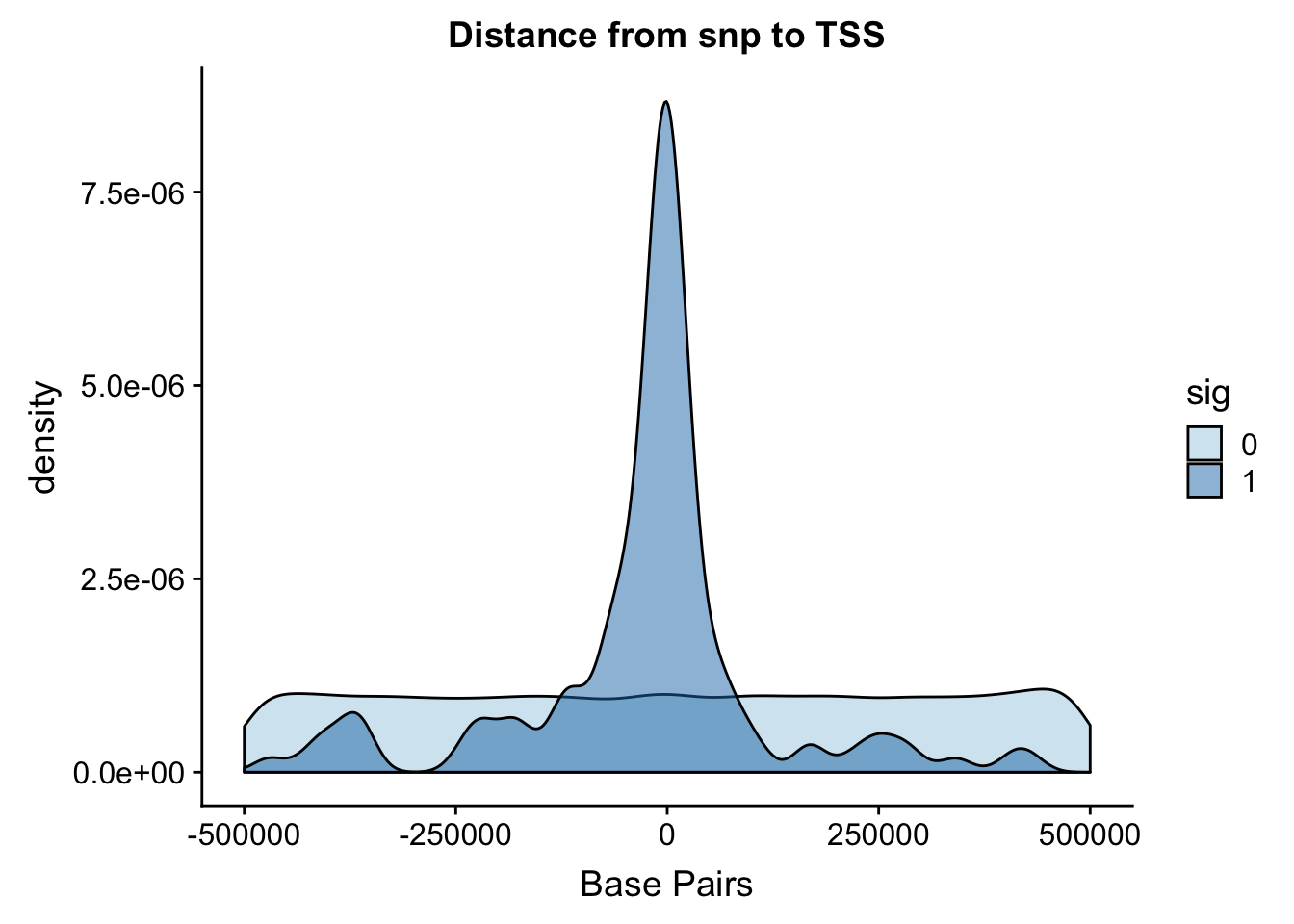
It looks like most of the signifcant values are 100,000 bases. This makes sense. I can zoom in on this portion.
ggplot(totalAPA, aes(x=dist, fill=sig, by=sig)) + geom_density(alpha=.5)+coord_cartesian(xlim = c(-150000, 150000)) + scale_fill_brewer(palette="Paired")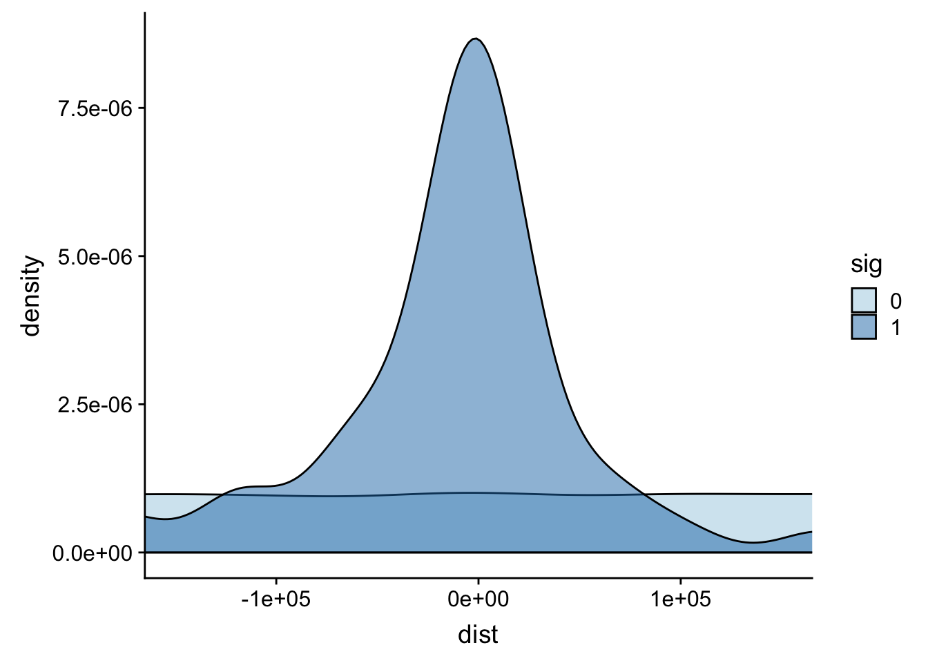
Distance from snp to peak
To perform this analysis I need to recover the peak positions.
The peak file I used for the QTL analysis is: /project2/gilad/briana/threeprimeseq/data/mergedPeaks_comb/filtered_APApeaks_merged_allchrom_refseqTrans.noties_sm.fixed.bed
peaks=read.table("../data/PeaksUsed/filtered_APApeaks_merged_allchrom_refseqTrans.noties_sm.fixed.bed", col.names = c("chr", "peakStart", "peakEnd", "PeakNum", "PeakScore", "Strand", "Gene")) %>% mutate(peak=paste("peak", PeakNum,sep="")) %>% mutate(PeakCenter=peakStart+ (peakEnd- peakStart))I want to join the peak start to the totalAPA file but the peak column. I will then create a column that is snppos-peakcenter.
totalAPA_peakdist= totalAPA %>%  inner_join(peaks, by="peak") %>%  separate(sid, into=c("snpCHR", "snpLOC"), by=":")
totalAPA_peakdist$snpLOC= as.numeric(totalAPA_peakdist$snpLOC)

totalAPA_peakdist= totalAPA_peakdist %>%  mutate(DisttoPeak= snpLOC-PeakCenter)
Plot this by significance.
ggplot(totalAPA_peakdist, aes(x=DisttoPeak, fill=sig, by=sig)) + geom_density(alpha=.5) + labs(title="Distance from snp peak", x="log10 absolute value Distance to Peak") + scale_fill_discrete(guide = guide_legend(title = "Significant QTL")) + scale_fill_brewer(palette="Paired")Scale for 'fill' is already present. Adding another scale for 'fill',
which will replace the existing scale.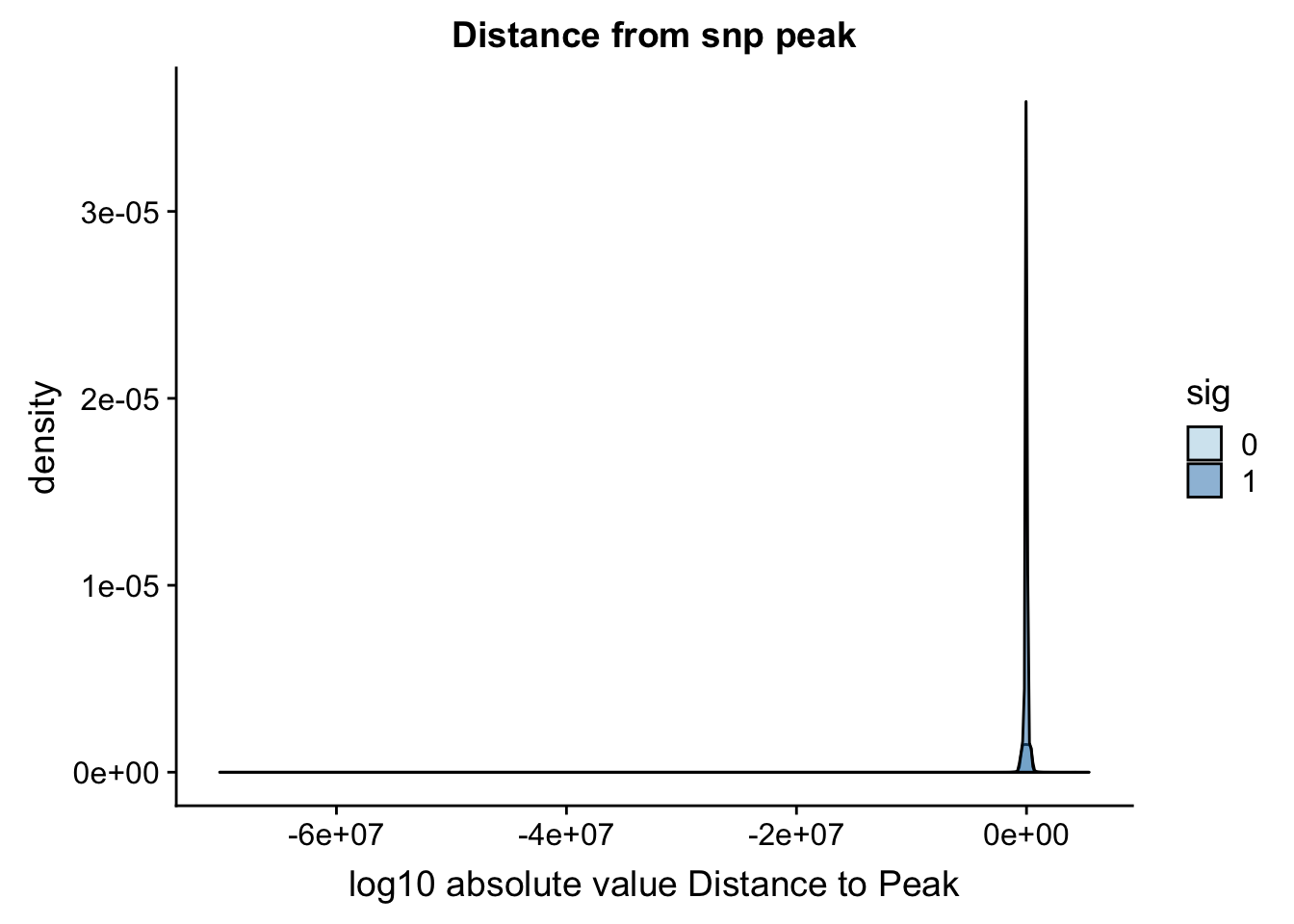
Look at the summarys based on significance:
totalAPA_peakdist_sig=totalAPA_peakdist %>% filter(sig==1)
totalAPA_peakdist_notsig=totalAPA_peakdist %>% filter(sig==0)


summary(totalAPA_peakdist_sig$DisttoPeak)
Min. 1st Qu. Median Mean 3rd Qu. Max.
-634474.0 -26505.0 -3325.5 -23883.8 492.5 460051.0 summary(totalAPA_peakdist_notsig$DisttoPeak) Min. 1st Qu. Median Mean 3rd Qu. Max.
-70147526 -269853 -1269 -6620 266370 5433999 ggplot(totalAPA_peakdist, aes(y=DisttoPeak,x=sig, fill=sig, by=sig)) + geom_boxplot() + scale_fill_discrete(guide = guide_legend(title = "Significant QTL")) + scale_fill_brewer(palette="Paired")Scale for 'fill' is already present. Adding another scale for 'fill',
which will replace the existing scale.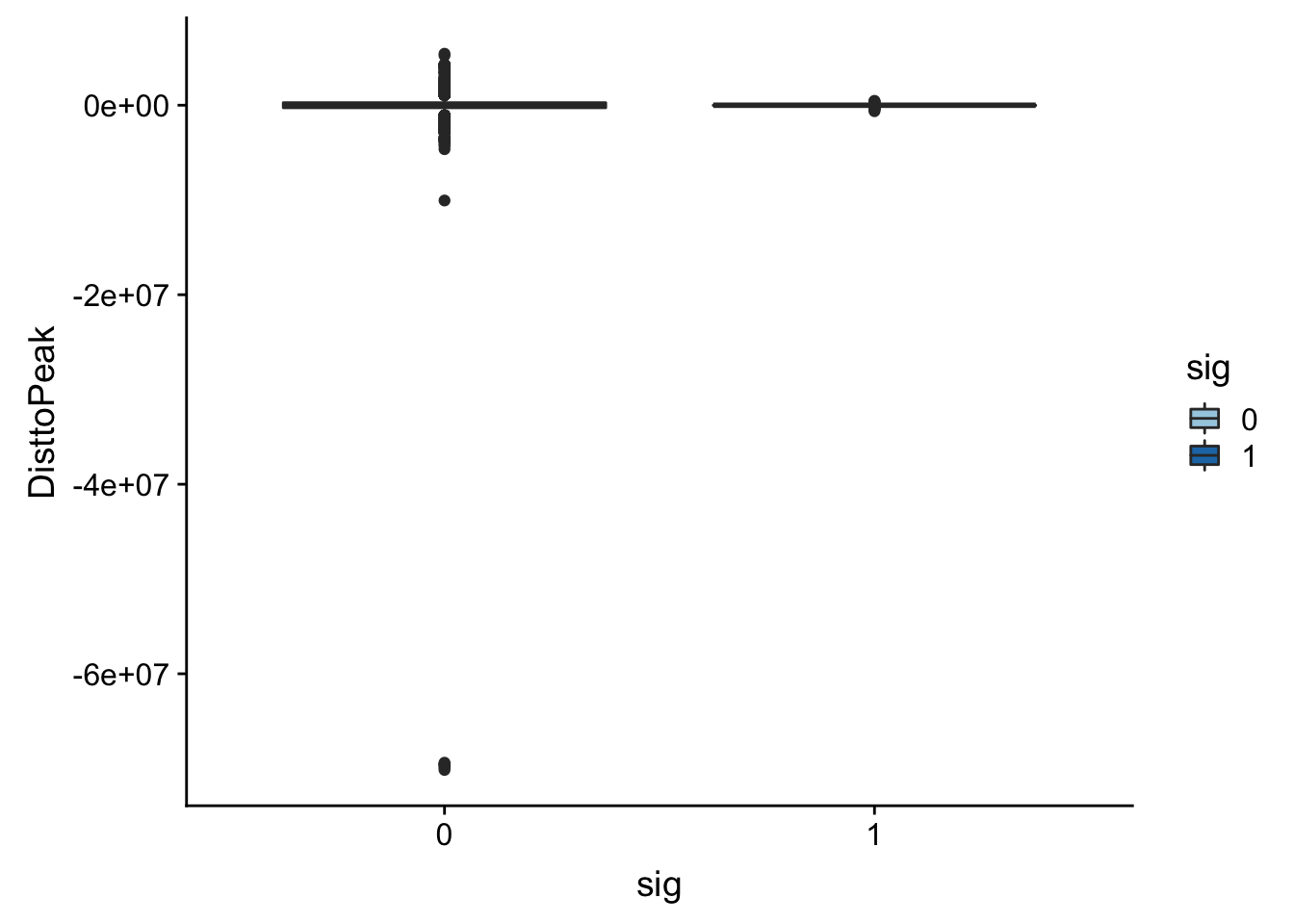
Look like there are some outliers that are really far. I will remove variants greater than 1*10^6th away
totalAPA_peakdist_filt=totalAPA_peakdist %>% filter(abs(DisttoPeak) <= 1*(10^6))

ggplot(totalAPA_peakdist_filt, aes(y=DisttoPeak,x=sig, fill=sig, by=sig)) + geom_boxplot()  + scale_fill_discrete(guide = guide_legend(title = "Significant QTL")) + facet_grid(.~strand) + scale_fill_brewer(palette="Paired")
Scale for 'fill' is already present. Adding another scale for 'fill',
which will replace the existing scale.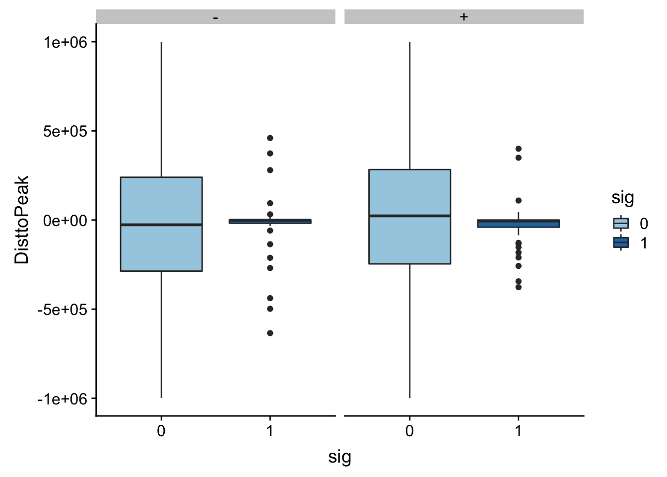
ggplot(totalAPA_peakdist_filt, aes(x=DisttoPeak, fill=sig, by=sig)) + geom_density() + scale_fill_discrete(guide = guide_legend(title = "Significant QTL")) + facet_grid(.~strand)+ scale_fill_brewer(palette="Paired")Scale for 'fill' is already present. Adding another scale for 'fill',
which will replace the existing scale.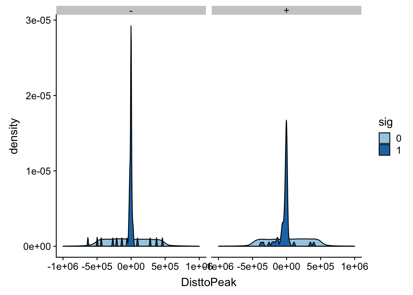
This gives a similar distribution.
I did snp - peak. This means if the peak is downstream of the snp on the positive strand the number will be negative.
In this case the peak is downstream of the snp.
totalAPA_peakdist %>% filter(sig==1) %>% filter(strand=="+") %>% filter(DisttoPeak < 0) %>% nrow()[1] 45totalAPA_peakdist %>% filter(sig==1) %>% filter(strand=="-") %>% filter(DisttoPeak > 0) %>% nrow()[1] 16Peak is upstream of the snp.
totalAPA_peakdist %>% filter(sig==1) %>% filter(strand=="+") %>% filter(DisttoPeak > 0) %>% nrow()[1] 17totalAPA_peakdist %>% filter(sig==1) %>% filter(strand=="-") %>% filter(DisttoPeak < 0) %>% nrow()[1] 40This means there is about 50/50 distribution around the peak start.
I am going to plot a violin plot for just the significant ones.
ggplot(totalAPA_peakdist_sig, aes(x=log10(abs(DisttoPeak)+1))) + geom_density(fill="darkviolet") + labs(title="Total: Distance from QTL to PAS Peak", x="Distance from SNP to PAS")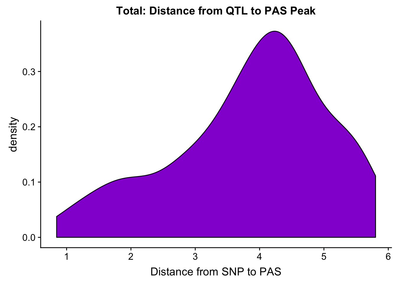
Within 1000 bases of the peak center.
totalAPA_peakdist_sig %>% filter(abs(DisttoPeak) < 1000) %>% nrow()[1] 29totalAPA_peakdist_sig %>% filter(abs(DisttoPeak) < 10000) %>% nrow()[1] 57totalAPA_peakdist_sig %>% filter(abs(DisttoPeak) < 100000) %>% nrow()[1] 9829 QTLs are within 1000 bp of the peak center, 57 within 10,000bp and 98 within 100,000bp
Expression metrics
Next I want to pull in the expression values and compare the expression of genes with a total APA qtl in comparison to genes without one. I will also need to pull in the gene names file to add in the gene names from the ensg ID.
Remove the # from the file.
expression=read.table("../data/mol_pheno/fastqtl_qqnorm_RNAseq_phase2.fixed.noChr.txt", header = T,stringsAsFactors = F)
expression_mean=apply(expression[,5:73],1,mean,na.rm=TRUE)
expression_var=apply(expression[,5:73],1,var,na.rm=TRUE)
expression$exp.mean= expression_mean
expression$exp.var=expression_var
expression= expression %>% separate(ID, into=c("Gene.stable.ID", "ver"), sep ="[.]")
Now I can pull in the names and join the dataframes.
geneNames=read.table("../data/ensemble_to_genename.txt", sep="\t", header=T,stringsAsFactors = F)


expression=expression %>% inner_join(geneNames,by="Gene.stable.ID")

expression=expression %>% select(Chr, start, end, Gene.name, exp.mean,exp.var) %>%  rename("gene"=Gene.name)
Now I can join this with the qtls.
totalAPA_wExp=totalAPA %>% inner_join(expression, by="gene") ggplot(totalAPA_wExp, aes(x=exp.mean, by=sig, fill=sig)) + geom_density(alpha=.3)+ scale_fill_brewer(palette="Paired")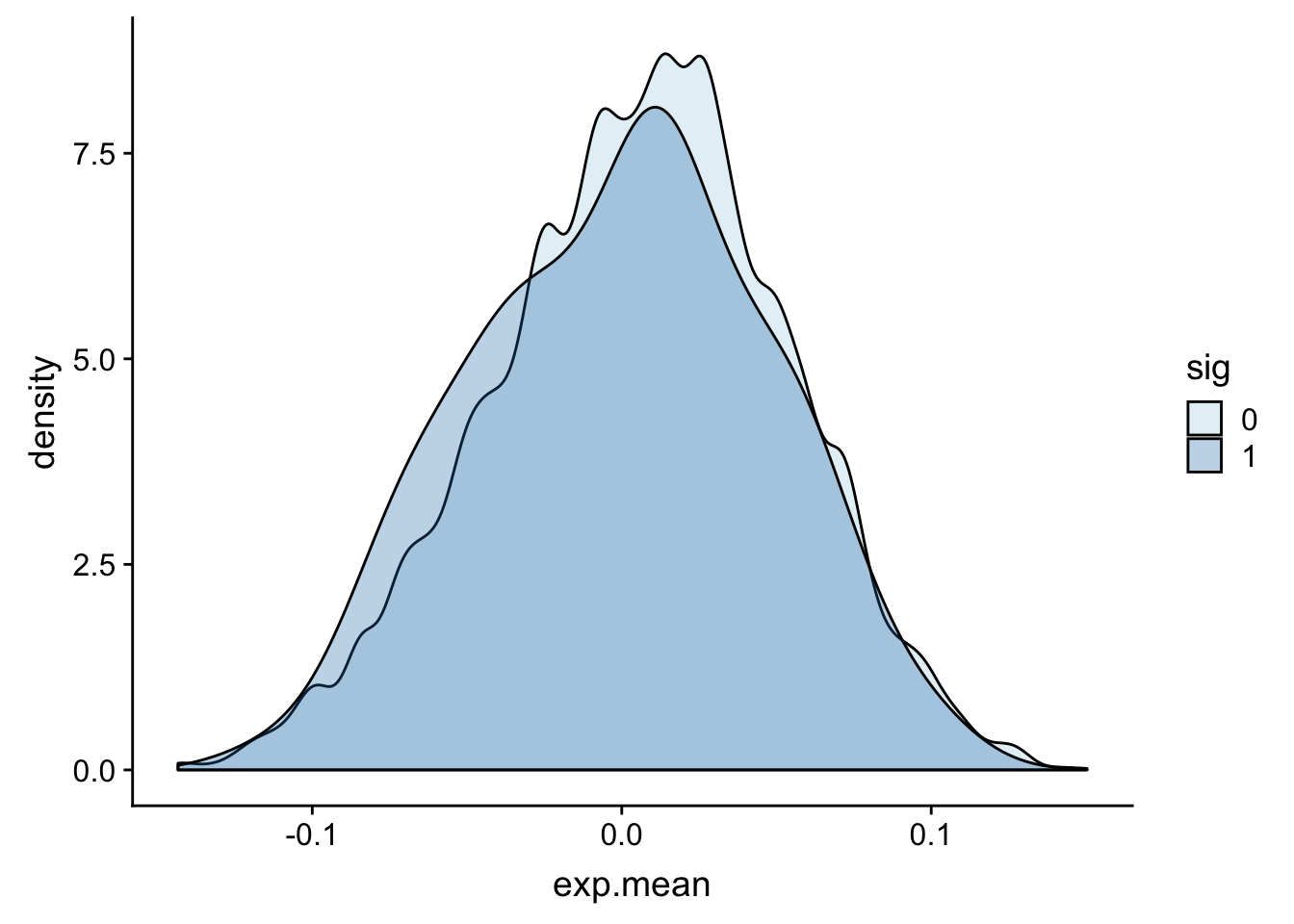
This is not exactly what I want because there are multiple peaks in a gene so some genes are plotted multiple times. I want to group the QTLs by gene and see if there is 1 sig QTL for that gene.
gene_wQTL= totalAPA_wExp %>% group_by(gene) %>% summarise(sig_gene=sum(as.numeric(as.character(sig)))) %>% ungroup() %>% inner_join(expression, by="gene") %>% mutate(sigGeneFactor=ifelse(sig_gene>=1, 1,0))

gene_wQTL$sigGeneFactor= as.factor(as.character(gene_wQTL$sigGeneFactor))
Therea are 92 genes in this set with a QTL.
ggplot(gene_wQTL, aes(x=exp.mean, by=sigGeneFactor, fill=sigGeneFactor)) + geom_density(alpha=.3) +labs(title="Mean in RNA expression by genes with significant QTL", x="Mean in normalized expression") + scale_fill_discrete(guide = guide_legend(title = "Significant QTL"))+ scale_fill_brewer(palette="Paired")Scale for 'fill' is already present. Adding another scale for 'fill',
which will replace the existing scale.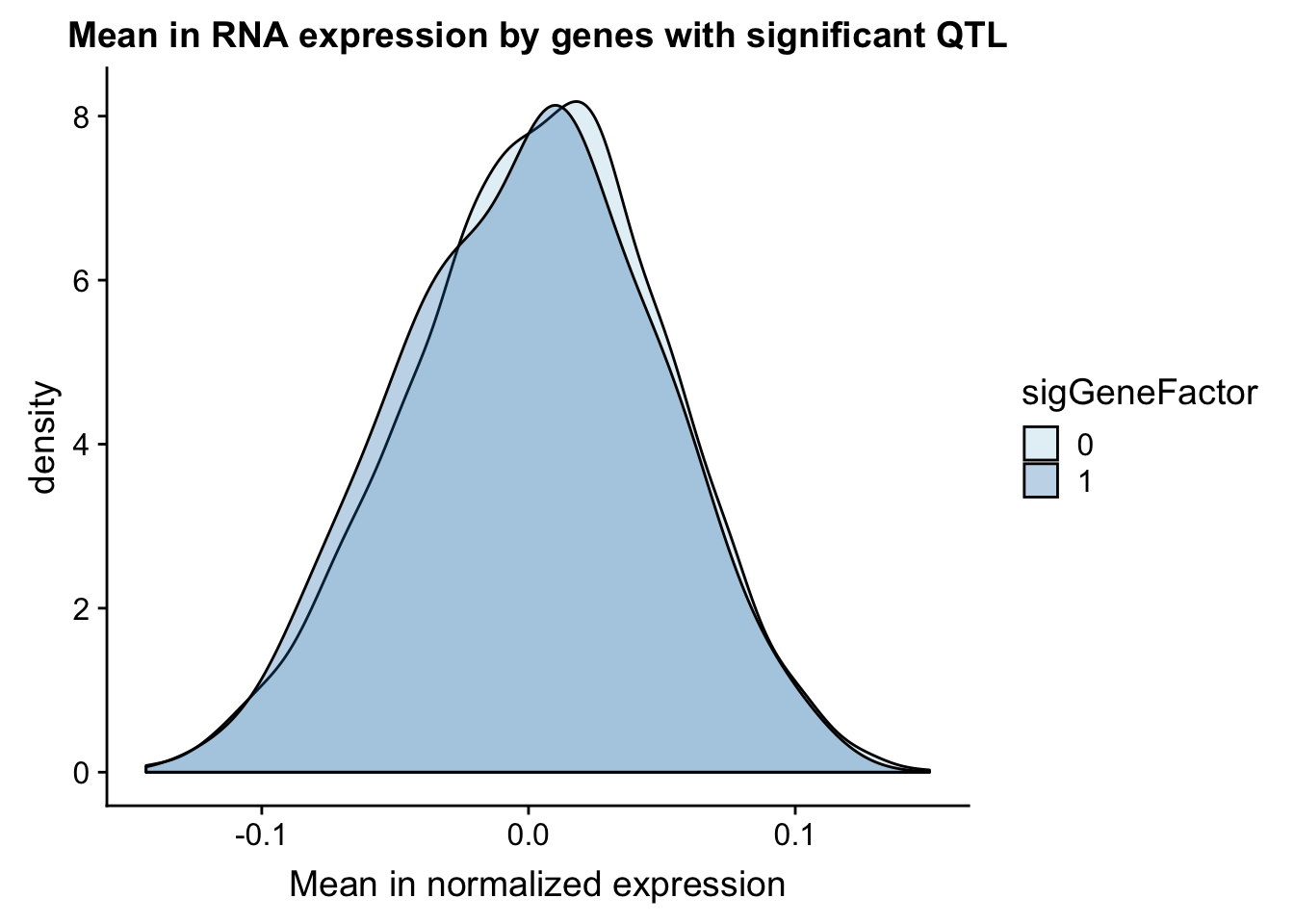
I can do a similar analysis but test the variance in the gene expression.
ggplot(gene_wQTL, aes(x=exp.var, by=sigGeneFactor, fill=sigGeneFactor)) + geom_density(alpha=.3) + labs(title="Varriance in RNA expression by genes with significant QTL", x="Variance in normalized expression") + scale_fill_discrete(guide = guide_legend(title = "Significant QTL"))+ scale_fill_brewer(palette="Paired")Scale for 'fill' is already present. Adding another scale for 'fill',
which will replace the existing scale.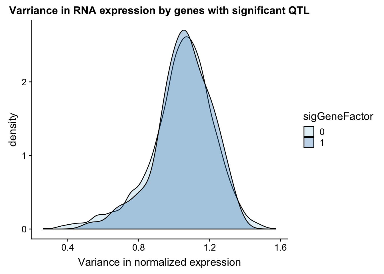
Peak coverage for QTLs
I can also look at peak coverage for peaks with QLTs and those without. I will first look at this on peak level then mvoe to gene level. The peak scores come from the coverage in the peaks.
The totalAPA_peakdist data frame has the information I need for this.
ggplot(totalAPA_peakdist, aes(x=PeakScore,fill=sig,by=sig)) + geom_density(alpha=.5)+ scale_x_log10() + labs(title="Peak score by significance") + scale_fill_brewer(palette="Paired")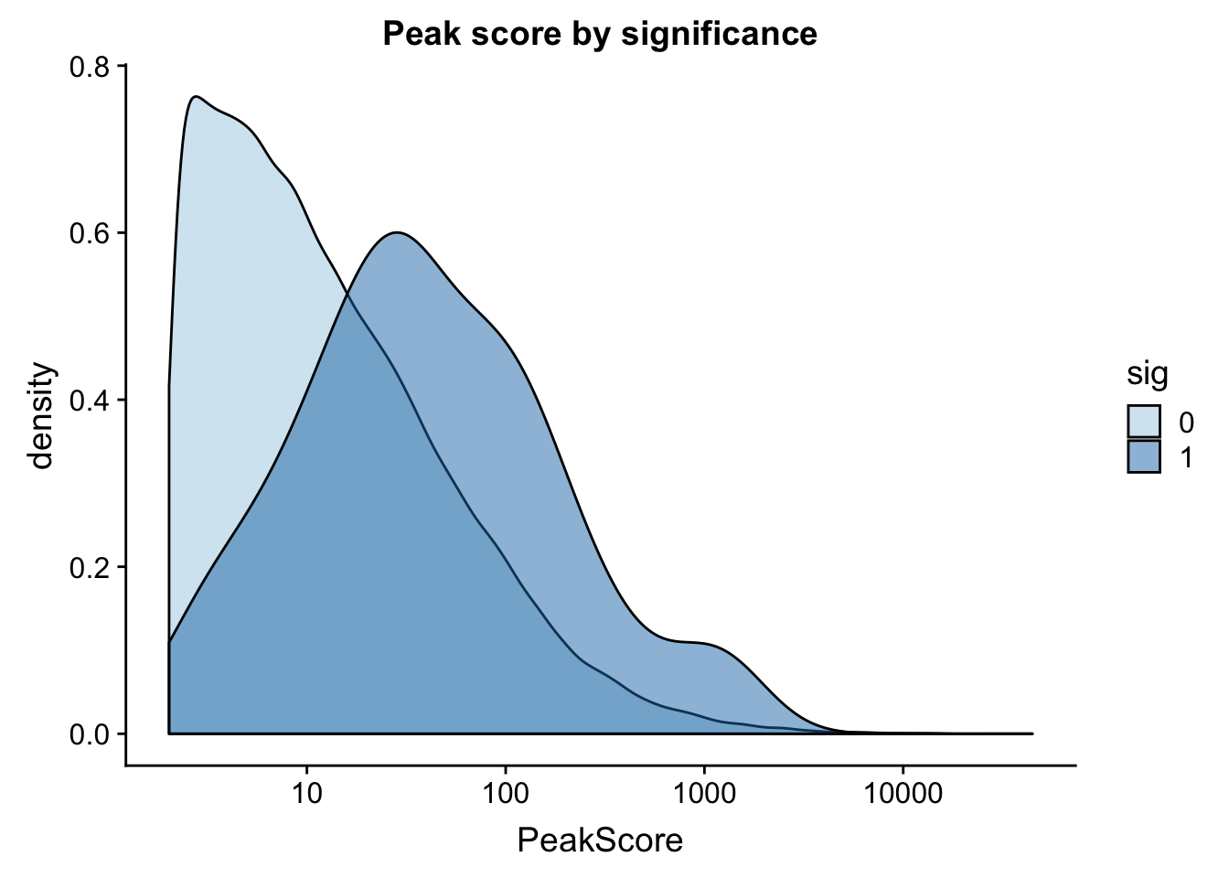
This is expected. It makes sense that we have more power to detect qtls in higher expressed peaks. This leads me to believe that filtering out low peaks may add power but will not mitigate the effect.
Where are the snps:
Download the GM12878 chromHMM annotation. I downleaded this from uscs and put it in:
- /Users/bmittleman1/Documents/Gilad_lab/threeprimeseq/data/GM12878.chromHMM.txt
- /project2/gilad/briana/genome_anotation_data/GM12878.chromHMM.txt
Column:
- bin
- chrom
- chromstart
- chromend
- name
- score
- strand
- thich start
- thick end
- item rgb
I can make this a bedfile to use a bedtools pipeline:
chrom (nochr)
start
end
name (txn hetero ect)
score
strand
fout = open("/project2/gilad/briana/genome_anotation_data/GM12878.chromHMM.bed",'w')
for ln in open("/project2/gilad/briana/genome_anotation_data/GM12878.chromHMM.txt", "r"):
    bin, chrom, start, end, name, score, strand, thSt, thE, rgb = ln.split()
    chrom=chrom[3:]
    name=name.split("_")[0]
    fout.write("%s\t%s\t%s\t%s\t%s\t%s\n"%(chrom, start, end, name, score, strand))
fout.close()
fout = open("/Users/bmittleman1/Documents/Gilad_lab/threeprimeseq/data/GM12878.chromHMM.bed",'w')
for ln in open("/Users/bmittleman1/Documents/Gilad_lab/threeprimeseq/data/GM12878.chromHMM.txt", "r"):
bin, chrom, start, end, name, score, strand, thSt, thE, rgb = ln.split()
chrom=chrom[3:]
fout.write("%s\t%s\t%s\t%s\t%s\t%s\n"%(chrom, start, end, name, score, strand))
fout.close()I also need to create a significant QTL snp bedfile for the total qtls. Bed files are 0 bases meaning I want the end to be the position I care about.
chrom, start (pos -1), end (pos), name, score (bh), strand
I can do this in python using the /project2/gilad/briana/threeprimeseq/data/perm_APAqtl_trans/filtered_APApeaks_merged_allchrom_refseqGenes_pheno_Total_transcript_permResBH.txt. I will make the script general to use on the total or nuclear file.
QTLres2SigSNPbed.py
def main(inFile, outFile):
    fout=open(outFile, "w")
    fin=open(inFile, "r")
    for num, ln in enumerate(fin):
      if num >= 1:
          pid, nvar, shape1, shape2, dummy, sid, dist, npval, slope, ppval, bpval, bh = ln.split()
          chrom, pos= sid.split(":")
          name=sid
          start= int(pos)-1
          end=int(pos)
          strand=pid.split(":")[3].split("_")[1]
          bh=float(bh)
          if bh <= .1:
              fout.write("%s\t%s\t%s\t%s\t%s\t%s\n"%(chrom, start, end, name, bh, strand))
    fout.close()

if __name__ == "__main__":
    import sys
    fraction=sys.argv[1]
    inFile = "/project2/gilad/briana/threeprimeseq/data/perm_APAqtl_trans/filtered_APApeaks_merged_allchrom_refseqGenes_pheno_%s_transcript_permResBH.txt"%(fraction)
    outFile= "/project2/gilad/briana/threeprimeseq/data/perm_APAqtl_trans/sigSnps/ApaQTLsignificantSnps_10percFDR_%s.bed"%(fraction)
    main(inFile,outFile)
I am going to try to use pybedtools instead for bedtools for this analysis. First I can add it to my conda environment.
Remove header from HMM
import pybedtools

sigNuc=pybedtools.BedTool('/project2/gilad/briana/threeprimeseq/data/perm_APAqtl_trans/sigSnps/ApaQTLsignificantSnps_10percFDR_Nuclear.sort.bed')

sigTot=pybedtools.BedTool('/project2/gilad/briana/threeprimeseq/data/perm_APAqtl_trans/sigSnps/ApaQTLsignificantSnps_10percFDR_Total.sort.bed')

hmm=pybedtools.BedTool("/project2/gilad/briana/genome_anotation_data/GM12878.chromHMM.sort.bed")

#map hmm to snps
Tot_overlapHMM=sigTot.map(hmm, c=4)

Nuc_overlapHMM=sigNuc.map(hmm,c=4)

#save results

Tot_overlapHMM.saveas("/project2/gilad/briana/threeprimeseq/data/perm_APAqtl_trans/sigSnps/Tot_overlapHMM.bed")

Nuc_overlapHMM.saveas("/project2/gilad/briana/threeprimeseq/data/perm_APAqtl_trans/sigSnps/Nuc_overlapHMM.bed")
I want to make a file that has all of the numbers for the chromatin regions for downstream analysis.
cut -f5 GM12878.chromHMM.txt | sort | uniq > chromHMM_regions.txtI then manually seperate the numbers from the name with a tab and remove the name line.
Evaluate results for total:
chromHmm=read.table("../data/ChromHmmOverlap/chromHMM_regions.txt", col.names = c("number", "name"), stringsAsFactors = F)

TotalOverlapHMM=read.table("../data/ChromHmmOverlap/Tot_overlapHMM.bed", col.names=c("chrom", "start", "end", "sid", "significance", "strand", "number"))

TotalOverlapHMM_names=TotalOverlapHMM %>% left_join(chromHmm, by="number")
ggplot(TotalOverlapHMM_names, aes(x=name)) + geom_bar() + labs(title="ChromHMM labels for Total APAQtls" , y="Number of SNPs", x="Region")+theme(axis.text.x = element_text(angle = 90, hjust = 1))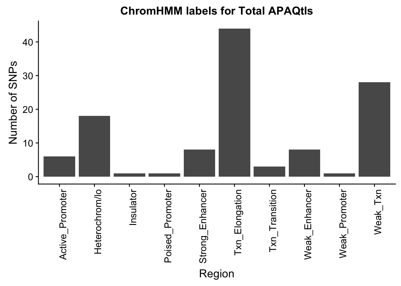
This is the count but I want enrichemnt. I need to randomly choose 188 snps from the ones I tested (nominal res) and get the same inforamtion on where they are.
shuf -n 118 /project2/gilad/briana/threeprimeseq/data/nominal_APAqtl_trans/filtered_APApeaks_merged_allchrom_refseqGenes_pheno_Total_NomRes.txt > /project2/gilad/briana/threeprimeseq/data/nominal_APAqtl_trans/randomSnps/ApaQTL_total_Random118.txt
Now I need to make these into the snp bed format.
QTLNOMres2SigSNPbed.py give this * total or nuclear
* number of snps
def main(inFile, outFile):
    fout=open(outFile, "w")
    fin=open(inFile, "r")
    for ln in fin:
          pid, sid, dist, pval, slope = ln.split()
          chrom, pos= sid.split(":")
          name=sid
          start= int(pos)-1
          end=int(pos)
          strand=pid.split(":")[3].split("_")[1]
          pval=float(pval)
          fout.write("%s\t%s\t%s\t%s\t%s\t%s\n"%(chrom, start, end, name, pval, strand))
    fout.close()

if __name__ == "__main__":
    import sys
    fraction=sys.argv[1]
    number=sys.argv[2]
    inFile = "/project2/gilad/briana/threeprimeseq/data/nominal_APAqtl_trans/randomSnps/ApaQTL_%s_Random%s.txt"%(fraction,number)
    outFile= "/project2/gilad/briana/threeprimeseq/data/nominal_APAqtl_trans/randomSnps/ApaQTL_%s_Random%s.bed"%(fraction,number)
    main(inFile,outFile)
Sort output
import pybedtools

RANDtot=pybedtools.BedTool('/project2/gilad/briana/threeprimeseq/data/nominal_APAqtl_trans/randomSnps/ApaQTL_total_Random118.sort.bed')


hmm=pybedtools.BedTool("/project2/gilad/briana/genome_anotation_data/GM12878.chromHMM.sort.bed")

#map hmm to snps
TotRnad_overlapHMM=RANDtot.map(hmm, c=4)


#save results

TotRnad_overlapHMM.saveas("/project2/gilad/briana/threeprimeseq/data/nominal_APAqtl_trans/randomSnps/ApaQTL_total_Random_overlapHMM.bed")
TotalRandOverlapHMM=read.table("../data/ChromHmmOverlap/ApaQTL_total_Random_overlapHMM.bed", col.names=c("chrom", "start", "end", "sid", "significance", "strand", "number"))

TotalRandOverlapHMM_names=TotalRandOverlapHMM %>% left_join(chromHmm, by="number")
ggplot(TotalRandOverlapHMM_names, aes(x=name)) + geom_bar() + labs(title="ChromHMM labels for Total APAQtls (Random)" , y="Number of SNPs", x="Region")+theme(axis.text.x = element_text(angle = 90, hjust = 1))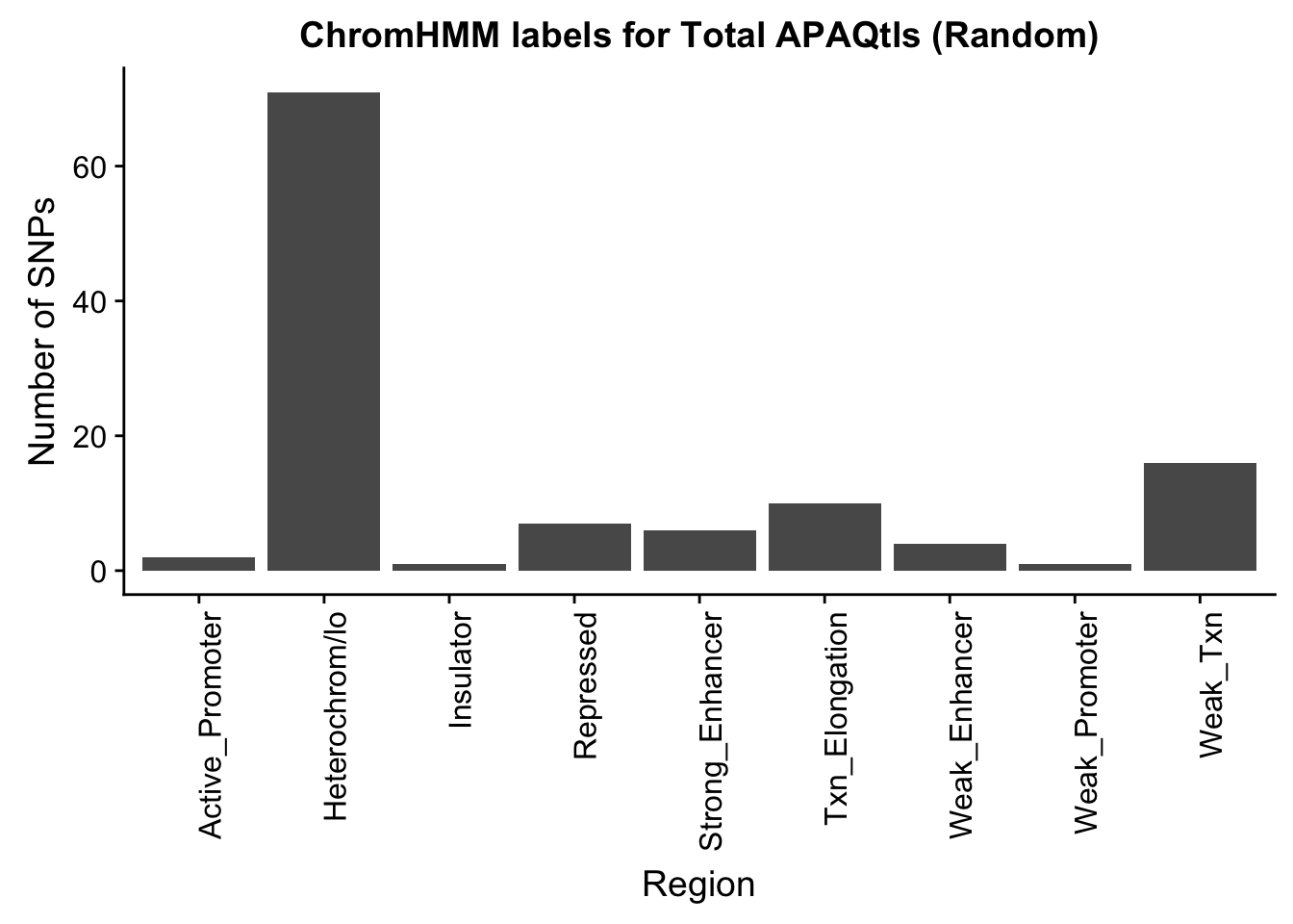
To put this on the same plot I can count the number in each then plot them next to eachother.
random_perChromHMM=TotalRandOverlapHMM_names %>%  group_by(name) %>% summarise(Random=n())
sig_perChromHMM= TotalOverlapHMM_names %>%  group_by(name) %>%  summarise(Total_QTLs=n())

perChrommHMM=random_perChromHMM %>%  full_join(sig_perChromHMM, by="name", ) %>% replace_na(list(Random=0,Total_QTLs=0))

perChrommHMM_melt=melt(perChrommHMM, id.vars="name")
names(perChrommHMM_melt)=c("Region","Set", "N_Snps" )
chromenrichTotalplot=ggplot(perChrommHMM_melt, aes(x=Region, y=N_Snps, by=Set, fill=Set)) + geom_bar(position="dodge", stat="identity") +theme(axis.text.x = element_text(angle = 90, hjust = 1)) + labs(title="Enrichment of Total QTLs by chromatin region", y="Number of Snps", x="Chromatin Region") + scale_fill_brewer(palette="Paired")
chromenrichTotalplot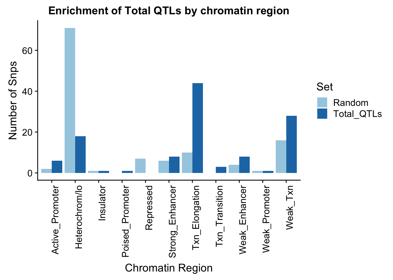
ggsave("../output/plots/ChromHmmEnrich_Total.png", chromenrichTotalplot)Saving 7 x 5 in imageI want to make a plot with the enrichment by fraction. I am first going to get an enrichemnt score for each bin naively by looking at the QTL-random in each category.
perChrommHMM$Random= as.integer(perChrommHMM$Random)
perChrommHMM$Total_QTLs= as.integer(perChrommHMM$Total_QTLs)
perChrommHMM_enr=perChrommHMM %>%  mutate(Total=Total_QTLs- Random)
Write this file so I can put it in the nuclear analysis and compare between groups.
write.table(perChrommHMM_enr, file="../data/ChromHmmOverlap/perChrommHMM_Total_enr.txt", quote=F, sep="\t", col.names = T, row.names = F)
sessionInfo()R version 3.5.1 (2018-07-02)
Platform: x86_64-apple-darwin15.6.0 (64-bit)
Running under: macOS 10.14.1
Matrix products: default
BLAS: /Library/Frameworks/R.framework/Versions/3.5/Resources/lib/libRblas.0.dylib
LAPACK: /Library/Frameworks/R.framework/Versions/3.5/Resources/lib/libRlapack.dylib
locale:
[1] en_US.UTF-8/en_US.UTF-8/en_US.UTF-8/C/en_US.UTF-8/en_US.UTF-8
attached base packages:
[1] grid stats graphics grDevices utils datasets methods
[8] base
other attached packages:
[1] bindrcpp_0.2.2 cowplot_0.9.3 data.table_1.11.8
[4] VennDiagram_1.6.20 futile.logger_1.4.3 forcats_0.3.0
[7] stringr_1.4.0 dplyr_0.7.6 purrr_0.2.5
[10] readr_1.1.1 tidyr_0.8.1 tibble_1.4.2
[13] ggplot2_3.0.0 tidyverse_1.2.1 reshape2_1.4.3
[16] workflowr_1.2.0
loaded via a namespace (and not attached):
[1] tidyselect_0.2.4 haven_1.1.2 lattice_0.20-35
[4] colorspace_1.3-2 htmltools_0.3.6 yaml_2.2.0
[7] rlang_0.2.2 pillar_1.3.0 glue_1.3.0
[10] withr_2.1.2 RColorBrewer_1.1-2 modelr_0.1.2
[13] lambda.r_1.2.3 readxl_1.1.0 bindr_0.1.1
[16] plyr_1.8.4 munsell_0.5.0 gtable_0.2.0
[19] cellranger_1.1.0 rvest_0.3.2 evaluate_0.13
[22] labeling_0.3 knitr_1.20 broom_0.5.0
[25] Rcpp_0.12.19 formatR_1.5 scales_1.0.0
[28] backports_1.1.2 jsonlite_1.6 fs_1.2.6
[31] hms_0.4.2 digest_0.6.17 stringi_1.2.4
[34] rprojroot_1.3-2 cli_1.0.1 tools_3.5.1
[37] magrittr_1.5 lazyeval_0.2.1 futile.options_1.0.1
[40] crayon_1.3.4 whisker_0.3-2 pkgconfig_2.0.2
[43] xml2_1.2.0 lubridate_1.7.4 assertthat_0.2.0
[46] rmarkdown_1.11 httr_1.3.1 rstudioapi_0.9.0
[49] R6_2.3.0 nlme_3.1-137 git2r_0.24.0
[52] compiler_3.5.1