Understand Peaks
Briana Mittleman
12/5/2018
Last updated: 2019-01-08
workflowr checks: (Click a bullet for more information)-
✔ R Markdown file: up-to-date
Great! Since the R Markdown file has been committed to the Git repository, you know the exact version of the code that produced these results.
-
✔ Environment: empty
Great job! The global environment was empty. Objects defined in the global environment can affect the analysis in your R Markdown file in unknown ways. For reproduciblity it’s best to always run the code in an empty environment.
-
✔ Seed:
set.seed(12345)The command
set.seed(12345)was run prior to running the code in the R Markdown file. Setting a seed ensures that any results that rely on randomness, e.g. subsampling or permutations, are reproducible. -
✔ Session information: recorded
Great job! Recording the operating system, R version, and package versions is critical for reproducibility.
-
Great! You are using Git for version control. Tracking code development and connecting the code version to the results is critical for reproducibility. The version displayed above was the version of the Git repository at the time these results were generated.✔ Repository version: 47f115d
Note that you need to be careful to ensure that all relevant files for the analysis have been committed to Git prior to generating the results (you can usewflow_publishorwflow_git_commit). workflowr only checks the R Markdown file, but you know if there are other scripts or data files that it depends on. Below is the status of the Git repository when the results were generated:
Note that any generated files, e.g. HTML, png, CSS, etc., are not included in this status report because it is ok for generated content to have uncommitted changes.Ignored files: Ignored: .DS_Store Ignored: .Rhistory Ignored: .Rproj.user/ Ignored: analysis/figure/ Ignored: data/.DS_Store Ignored: output/.DS_Store Untracked files: Untracked: KalistoAbundance18486.txt Untracked: analysis/DirectionapaQTL.Rmd Untracked: analysis/ncbiRefSeq_sm.sort.mRNA.bed Untracked: analysis/snake.config.notes.Rmd Untracked: analysis/verifyBAM.Rmd Untracked: code/PeaksToCoverPerReads.py Untracked: code/strober_pc_pve_heatmap_func.R Untracked: data/18486.genecov.txt Untracked: data/APApeaksYL.total.inbrain.bed Untracked: data/ChromHmmOverlap/ Untracked: data/GM12878.chromHMM.bed Untracked: data/GM12878.chromHMM.txt Untracked: data/LianoglouLCL/ Untracked: data/LocusZoom/ Untracked: data/NuclearApaQTLs.txt Untracked: data/PeakCounts/ Untracked: data/PeaksUsed/ Untracked: data/RNAkalisto/ Untracked: data/TotalApaQTLs.txt Untracked: data/Totalpeaks_filtered_clean.bed Untracked: data/UnderstandPeaksQC/ Untracked: data/YL-SP-18486-T-combined-genecov.txt Untracked: data/YL-SP-18486-T_S9_R1_001-genecov.txt Untracked: data/apaExamp/ Untracked: data/bedgraph_peaks/ Untracked: data/bin200.5.T.nuccov.bed Untracked: data/bin200.Anuccov.bed Untracked: data/bin200.nuccov.bed Untracked: data/clean_peaks/ Untracked: data/comb_map_stats.csv Untracked: data/comb_map_stats.xlsx Untracked: data/comb_map_stats_39ind.csv Untracked: data/combined_reads_mapped_three_prime_seq.csv Untracked: data/diff_iso_trans/ Untracked: data/ensemble_to_genename.txt Untracked: data/example_gene_peakQuant/ Untracked: data/explainProtVar/ Untracked: data/filtered_APApeaks_merged_allchrom_refseqTrans.closest2End.bed Untracked: data/filtered_APApeaks_merged_allchrom_refseqTrans.closest2End.noties.bed Untracked: data/first50lines_closest.txt Untracked: data/gencov.test.csv Untracked: data/gencov.test.txt Untracked: data/gencov_zero.test.csv Untracked: data/gencov_zero.test.txt Untracked: data/gene_cov/ Untracked: data/joined Untracked: data/leafcutter/ Untracked: data/merged_combined_YL-SP-threeprimeseq.bg Untracked: data/mol_overlap/ Untracked: data/mol_pheno/ Untracked: data/nom_QTL/ Untracked: data/nom_QTL_opp/ Untracked: data/nom_QTL_trans/ Untracked: data/nuc6up/ Untracked: data/other_qtls/ Untracked: data/pQTL_otherphen/ Untracked: data/peakPerRefSeqGene/ Untracked: data/perm_QTL/ Untracked: data/perm_QTL_opp/ Untracked: data/perm_QTL_trans/ Untracked: data/perm_QTL_trans_filt/ Untracked: data/reads_mapped_three_prime_seq.csv Untracked: data/smash.cov.results.bed Untracked: data/smash.cov.results.csv Untracked: data/smash.cov.results.txt Untracked: data/smash_testregion/ Untracked: data/ssFC200.cov.bed Untracked: data/temp.file1 Untracked: data/temp.file2 Untracked: data/temp.gencov.test.txt Untracked: data/temp.gencov_zero.test.txt Untracked: data/threePrimeSeqMetaData.csv Untracked: output/picard/ Untracked: output/plots/ Untracked: output/qual.fig2.pdf Unstaged changes: Modified: analysis/28ind.peak.explore.Rmd Modified: analysis/InvestigatePeak2GeneAssignment.Rmd Modified: analysis/apaQTLoverlapGWAS.Rmd Modified: analysis/cleanupdtseq.internalpriming.Rmd Modified: analysis/coloc_apaQTLs_protQTLs.Rmd Modified: analysis/dif.iso.usage.leafcutter.Rmd Modified: analysis/diff_iso_pipeline.Rmd Modified: analysis/explainpQTLs.Rmd Modified: analysis/explore.filters.Rmd Modified: analysis/flash2mash.Rmd Modified: analysis/overlapMolQTL.Rmd Modified: analysis/overlap_qtls.Rmd Modified: analysis/peakOverlap_oppstrand.Rmd Modified: analysis/pheno.leaf.comb.Rmd Modified: analysis/swarmPlots_QTLs.Rmd Modified: analysis/test.max2.Rmd Modified: code/Snakefile
Expand here to see past versions:
| File | Version | Author | Date | Message |
|---|---|---|---|---|
| Rmd | 47f115d | Briana Mittleman | 2019-01-08 | code for deeptools plots |
| html | 6da90e9 | Briana Mittleman | 2018-12-11 | Build site. |
| Rmd | 035053c | Briana Mittleman | 2018-12-11 | work on peak and gene assignments |
| html | afafcc3 | Briana Mittleman | 2018-12-10 | Build site. |
| Rmd | bc9f4cf | Briana Mittleman | 2018-12-10 | add plot 2 peaks to get perc reads |
| html | 1549daf | Briana Mittleman | 2018-12-07 | Build site. |
| Rmd | 38843d3 | Briana Mittleman | 2018-12-07 | update q2 with current problem |
| html | daa5818 | Briana Mittleman | 2018-12-07 | Build site. |
| Rmd | fa26526 | Briana Mittleman | 2018-12-07 | add filter correlation |
| html | 7848485 | Briana Mittleman | 2018-12-07 | Build site. |
| Rmd | 55c61ea | Briana Mittleman | 2018-12-07 | scatterplot TPM vs gene cov |
| html | 3cd438e | Briana Mittleman | 2018-12-06 | Build site. |
| Rmd | ddde22b | Briana Mittleman | 2018-12-06 | add peaks per feature plot |
| html | cdfa5b2 | Briana Mittleman | 2018-12-05 | Build site. |
| Rmd | 655b582 | Briana Mittleman | 2018-12-05 | PCA with batch and read count |
The goal of this analysis is to understand the data a bit better at the peak level. I want to have the cleanest set of peaks when I perform the final anlyses for the paper.
Variation in peaks
First I will run PCA on the peak coverage. I will run this seperatly for the total and nuclear fractions. I do not expect large amount of separation.
I will use the peak coverage data before the ratios are created for leafcutter. These files were created using feature counts on the filtered peaks. At this point the peaks have been mapped to the closest refseq transcript on the opposite strand.
Relevant file:
* /project2/gilad/briana/threeprimeseq/data/filtPeakOppstrand_cov/filtered_APApeaks_merged_allchrom_refseqGenes.Transcript_sm_quant.Total_fixed.fc
- /project2/gilad/briana/threeprimeseq/data/filtPeakOppstrand_cov/filtered_APApeaks_merged_allchrom_refseqGenes.Transcript_sm_quant.Nuclear_fixed.fc
These files are in /Users/bmittleman1/Documents/Gilad_lab/threeprimeseq/data/PeakCounts on my computer.
library(tidyverse)── Attaching packages ──────────────────────────────────────────────────── tidyverse 1.2.1 ──✔ ggplot2 3.0.0 ✔ purrr 0.2.5
✔ tibble 1.4.2 ✔ dplyr 0.7.6
✔ tidyr 0.8.1 ✔ stringr 1.3.1
✔ readr 1.1.1 ✔ forcats 0.3.0── Conflicts ─────────────────────────────────────────────────────── tidyverse_conflicts() ──
✖ dplyr::filter() masks stats::filter()
✖ dplyr::lag() masks stats::lag()library(workflowr)This is workflowr version 1.1.1
Run ?workflowr for help getting startedlibrary(cowplot)
Attaching package: 'cowplot'The following object is masked from 'package:ggplot2':
ggsavelibrary(reshape2)
Attaching package: 'reshape2'The following object is masked from 'package:tidyr':
smithslibrary(devtools)
library(tximport)Load data:
#only keep the counts
total_Cov=read.table("../data/PeakCounts/filtered_APApeaks_merged_allchrom_refseqGenes.Transcript_sm_quant.Total_fixed.fc", header=T, stringsAsFactors = F)[,7:45]
nuclear_Cov=read.table("../data/PeakCounts/filtered_APApeaks_merged_allchrom_refseqGenes.Transcript_sm_quant.Nuclear_fixed.fc", header=T, stringsAsFactors = F)[,7:45]
ggplot(total_Cov, aes(x=log10(X18486_T))) + geom_density()Warning: Removed 233009 rows containing non-finite values (stat_density).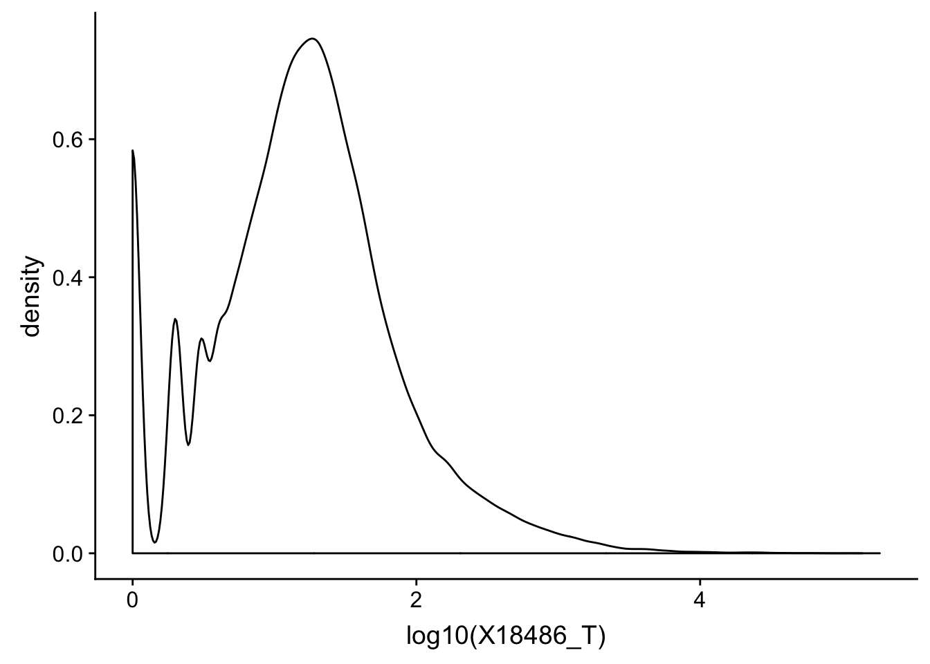
Expand here to see past versions of unnamed-chunk-3-1.png:
| Version | Author | Date |
|---|---|---|
| afafcc3 | Briana Mittleman | 2018-12-10 |
Total:
Run PCA on the total coverage
pca_tot_peak=prcomp(total_Cov, center=T,scale=T)
summary(pca_tot_peak)
Importance of components:
PC1 PC2 PC3 PC4 PC5 PC6
Standard deviation 5.9010 1.30000 0.81376 0.75658 0.47993 0.4501
Proportion of Variance 0.8929 0.04333 0.01698 0.01468 0.00591 0.0052
Cumulative Proportion 0.8929 0.93621 0.95319 0.96787 0.97378 0.9790
PC7 PC8 PC9 PC10 PC11 PC12
Standard deviation 0.42896 0.32313 0.30419 0.27984 0.23427 0.19916
Proportion of Variance 0.00472 0.00268 0.00237 0.00201 0.00141 0.00102
Cumulative Proportion 0.98369 0.98637 0.98874 0.99075 0.99216 0.99317
PC13 PC14 PC15 PC16 PC17 PC18
Standard deviation 0.18883 0.15913 0.15127 0.14309 0.12758 0.1254
Proportion of Variance 0.00091 0.00065 0.00059 0.00053 0.00042 0.0004
Cumulative Proportion 0.99409 0.99474 0.99532 0.99585 0.99626 0.9967
PC19 PC20 PC21 PC22 PC23 PC24
Standard deviation 0.12328 0.11035 0.10707 0.09979 0.09530 0.08797
Proportion of Variance 0.00039 0.00031 0.00029 0.00026 0.00023 0.00020
Cumulative Proportion 0.99706 0.99737 0.99766 0.99792 0.99815 0.99835
PC25 PC26 PC27 PC28 PC29 PC30
Standard deviation 0.08576 0.08086 0.07902 0.07535 0.07454 0.06907
Proportion of Variance 0.00019 0.00017 0.00016 0.00015 0.00014 0.00012
Cumulative Proportion 0.99854 0.99871 0.99887 0.99901 0.99916 0.99928
PC31 PC32 PC33 PC34 PC35 PC36
Standard deviation 0.06717 0.06441 0.06201 0.05666 0.05415 0.05261
Proportion of Variance 0.00012 0.00011 0.00010 0.00008 0.00008 0.00007
Cumulative Proportion 0.99939 0.99950 0.99960 0.99968 0.99976 0.99983
PC37 PC38 PC39
Standard deviation 0.05128 0.04839 0.04237
Proportion of Variance 0.00007 0.00006 0.00005
Cumulative Proportion 0.99989 0.99995 1.00000pca_tot_df=as.data.frame(pca_tot_peak$rotation) %>% rownames_to_column(var="lib") %>% mutate(line=substr(lib,2,6))
pca_tot_df$line=as.integer(pca_tot_df$line)I want to color these by library size.
map_stats=read.csv("../data/comb_map_stats_39ind.csv", header=T)

map_stat_total=map_stats %>% filter(fraction=="total")
map_stat_total$batch=as.factor(map_stat_total$batch)
Join the relevant stats with the pca dataframe.
pca_tot_df=pca_tot_df %>% full_join(map_stat_total, by="line")Plot this PCA:
totPCA_batch=ggplot(pca_tot_df, aes(x=PC1, y=PC2, col=batch )) + geom_point() + labs(x="PC1:0.89", y="PC2:0.043", title="Raw PAS qunatification data Total \n colored by batch ")
ggsave("../output/plots/QC_plots/TotalPCA_colBatch.png",totPCA_batch)
Saving 7 x 5 in imagetotPCA_mapped=ggplot(pca_tot_df, aes(x=PC1, y=PC2, col=comb_mapped )) + geom_point() + labs(x="PC1:0.89", y="PC2:0.043", title="Raw PAS qunatification data Total \n colored by Mapped Read count")
ggsave("../output/plots/QC_plots/TotalPCA_colMapped.png",totPCA_mapped)Saving 7 x 5 in imageNuclear
Run PCA on the Nuclear coverage
pca_nuc_peak=prcomp(nuclear_Cov, center=T,scale=T)
summary(pca_nuc_peak)
Importance of components:
PC1 PC2 PC3 PC4 PC5 PC6
Standard deviation 5.3861 1.87775 1.62240 0.99268 0.92998 0.63513
Proportion of Variance 0.7438 0.09041 0.06749 0.02527 0.02218 0.01034
Cumulative Proportion 0.7438 0.83425 0.90174 0.92701 0.94919 0.95953
PC7 PC8 PC9 PC10 PC11 PC12
Standard deviation 0.53149 0.4674 0.4095 0.36160 0.32862 0.28960
Proportion of Variance 0.00724 0.0056 0.0043 0.00335 0.00277 0.00215
Cumulative Proportion 0.96677 0.9724 0.9767 0.98003 0.98280 0.98495
PC13 PC14 PC15 PC16 PC17 PC18
Standard deviation 0.26862 0.25414 0.2333 0.22825 0.20329 0.19277
Proportion of Variance 0.00185 0.00166 0.0014 0.00134 0.00106 0.00095
Cumulative Proportion 0.98680 0.98845 0.9899 0.99118 0.99224 0.99320
PC19 PC20 PC21 PC22 PC23 PC24
Standard deviation 0.18620 0.17247 0.16092 0.14244 0.13630 0.12741
Proportion of Variance 0.00089 0.00076 0.00066 0.00052 0.00048 0.00042
Cumulative Proportion 0.99409 0.99485 0.99551 0.99603 0.99651 0.99693
PC25 PC26 PC27 PC28 PC29 PC30
Standard deviation 0.12025 0.11377 0.11306 0.10563 0.10228 0.09219
Proportion of Variance 0.00037 0.00033 0.00033 0.00029 0.00027 0.00022
Cumulative Proportion 0.99730 0.99763 0.99796 0.99824 0.99851 0.99873
PC31 PC32 PC33 PC34 PC35 PC36
Standard deviation 0.08916 0.08768 0.08144 0.07916 0.07412 0.07253
Proportion of Variance 0.00020 0.00020 0.00017 0.00016 0.00014 0.00013
Cumulative Proportion 0.99893 0.99913 0.99930 0.99946 0.99960 0.99974
PC37 PC38 PC39
Standard deviation 0.06394 0.05721 0.05416
Proportion of Variance 0.00010 0.00008 0.00008
Cumulative Proportion 0.99984 0.99992 1.00000pca_nuc_df=as.data.frame(pca_nuc_peak$rotation) %>% rownames_to_column(var="lib") %>% mutate(line=substr(lib,2,6))
pca_nuc_df$line=as.integer(pca_nuc_df$line)I want to color these by library size.
map_stat_nuclear=map_stats %>% filter(fraction=="nuclear")
map_stat_nuclear$batch=as.factor(map_stat_nuclear$batch)
Join the relevant stats with the pca dataframe.
pca_nuc_df=pca_nuc_df %>% full_join(map_stat_nuclear, by="line")Plot this PCA:
nucPCA_batch=ggplot(pca_nuc_df, aes(x=PC1, y=PC2, col=batch )) + geom_point() + labs(x="PC1: 0.74", y="PC2: 0.09", title="Raw PAS qunatification data nuclear \n colored by batch ")
ggsave("../output/plots/QC_plots/NuclearPCA_colBatch.png",nucPCA_batch)
Saving 7 x 5 in imageThis shows that PC 2 is highly corrleated with batch,
nucPCA_mapped=ggplot(pca_nuc_df, aes(x=PC1, y=PC2, col=comb_mapped )) + geom_point() + labs(x="PC1: 0.74", y="PC2: 0.09", title="Raw PAS qunatification data nuclear \n colored by Mapped Read count")
ggsave("../output/plots/QC_plots/NuclearlPCA_colMapped.png",nucPCA_mapped)
Saving 7 x 5 in imageQ: Do the PAS read number recapitulate gene expression as it should?
Plot: scatter plot + fit (x-axis: gene TPM, y-axis: gene normalized PAS counts) total/nuclear separate
The TPM measurements come from the kalisto run I did on 18486.
tx2gene=read.table("../data/RNAkalisto/ncbiRefSeq.txn2gene.txt" ,header= F, sep="\t", stringsAsFactors = F)

txi.kallisto.tsv <- tximport("../data/RNAkalisto/abundance.tsv", type = "kallisto", tx2gene = tx2gene,countsFromAbundance="lengthScaledTPM" )
Note: importing `abundance.h5` is typically faster than `abundance.tsv`reading in files with read_tsv1
removing duplicated transcript rows from tx2gene
transcripts missing from tx2gene: 99
summarizing abundance
summarizing counts
summarizing lengthI need to get all of the peaks for 18486 and which gene they are in. Then I will take the gene average and divide by the number of mapped reads.
total_Cov_18486=read.table("../data/PeakCounts/filtered_APApeaks_merged_allchrom_refseqGenes.Transcript_sm_quant.Total_fixed.fc", header=T, stringsAsFactors = F)[,1:7] %>% separate(Geneid, into=c("peak", "chr", "start", "end", "strand", "gene"), sep=":") %>% select(gene, X18486_T) %>% filter(X18486_T>10) %>%  group_by(gene) %>% summarize(GeneSum=sum(X18486_T)) %>% mutate(GeneSumNorm=GeneSum/10.8)

#%>% mutate(NormGenePeakCov=GeneSum/10819437)
Join with the transcript TPM
TXN_abund=as.data.frame(txi.kallisto.tsv$abundance) %>% rownames_to_column(var="gene")
colnames(TXN_abund)=c("gene", "TPM")

TXN_NormGene=TXN_abund %>% inner_join(total_Cov_18486,by="gene")
Plot distribution of each variable seperatly first to understand distribution:
summary(TXN_abund$TPM) Min. 1st Qu. Median Mean 3rd Qu. Max.
0.00 0.02 1.03 36.87 14.21 101438.00 ggplot(TXN_abund, aes(x=log10(TPM))) + geom_density(kernel="gaussian") + scale_x_log10()Warning in self$trans$transform(x): NaNs producedWarning: Transformation introduced infinite values in continuous x-axisWarning: Removed 13505 rows containing non-finite values (stat_density).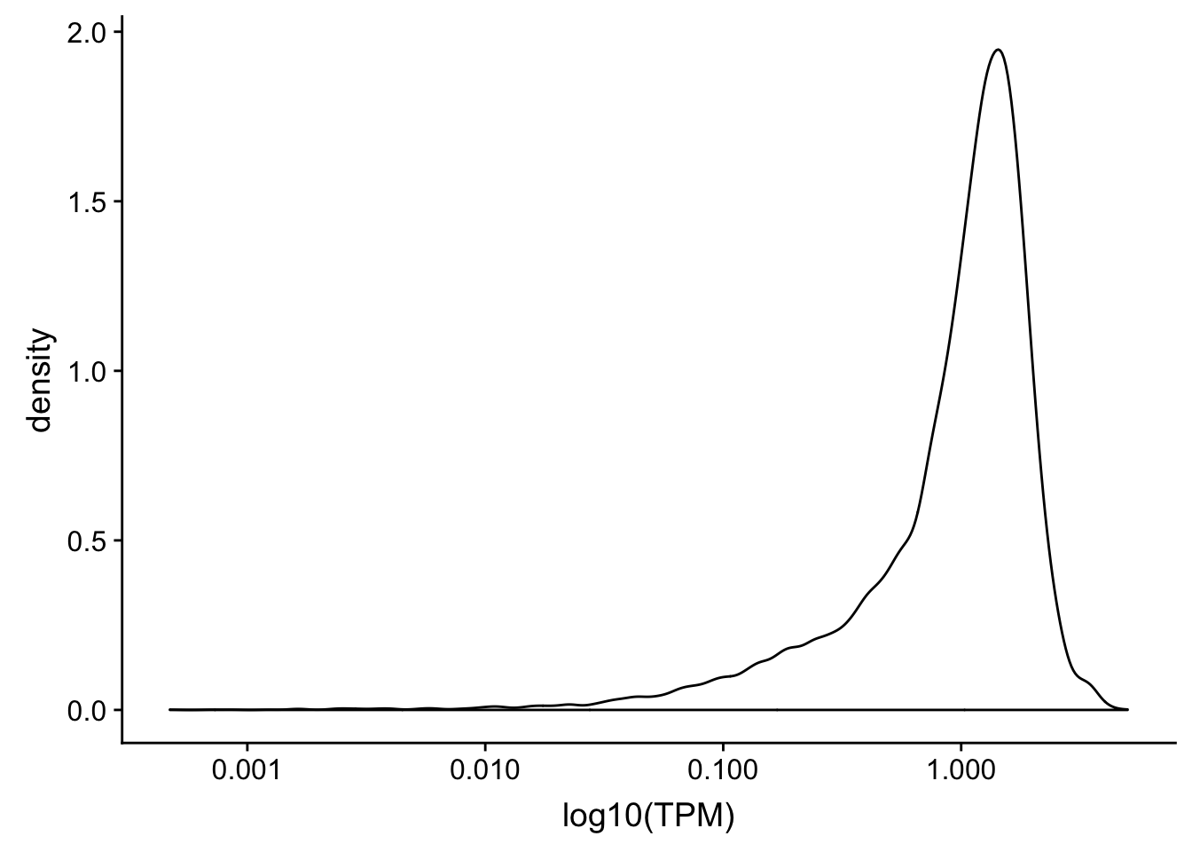
Expand here to see past versions of unnamed-chunk-16-1.png:
| Version | Author | Date |
|---|---|---|
| 6da90e9 | Briana Mittleman | 2018-12-11 |
| afafcc3 | Briana Mittleman | 2018-12-10 |
| daa5818 | Briana Mittleman | 2018-12-07 |
| 7848485 | Briana Mittleman | 2018-12-07 |
summary(total_Cov_18486$GeneSumNorm) Min. 1st Qu. Median Mean 3rd Qu. Max.
1.019 7.963 22.963 68.164 56.551 17110.648 ggplot(total_Cov_18486, aes(x=log10(GeneSumNorm))) + geom_density(kernel="gaussian")+ scale_x_log10()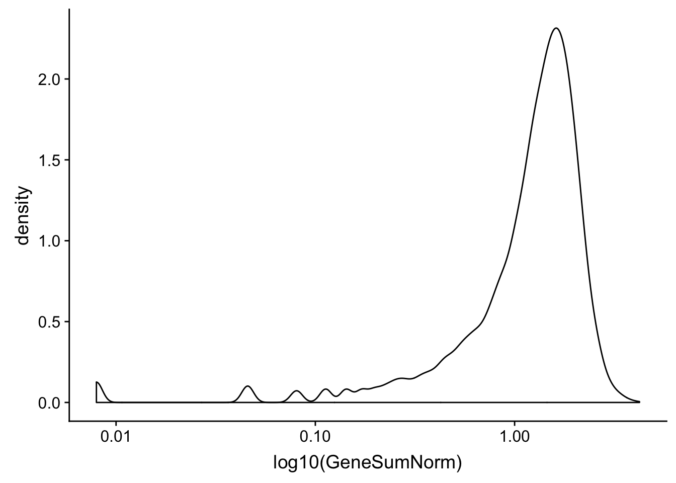
Expand here to see past versions of unnamed-chunk-17-1.png:
| Version | Author | Date |
|---|---|---|
| 6da90e9 | Briana Mittleman | 2018-12-11 |
| afafcc3 | Briana Mittleman | 2018-12-10 |
| 7848485 | Briana Mittleman | 2018-12-07 |
| 3cd438e | Briana Mittleman | 2018-12-06 |
Create a scatterplot:
TXN_NormGene=TXN_NormGene %>% filter(TPM>0) %>% filter(GeneSumNorm>0)
corr_18486Tot=ggplot(TXN_NormGene, aes(x=log10(TPM), y= log10(GeneSumNorm))) + geom_point() + labs(title="Total", x="log10 RNA seq TPM", y="log10 Peak count sum per gene")+ geom_smooth(aes(x=log10(TPM),y=log10(GeneSumNorm)),method = "lm") + annotate("text",x=5, y=5,label="R2=.42")+ geom_text(aes(label=gene),hjust=0, vjust=0)

corr_18486Tot 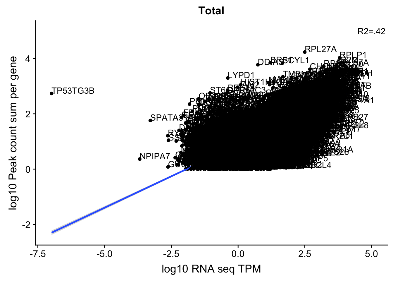
Expand here to see past versions of unnamed-chunk-18-1.png:
| Version | Author | Date |
|---|---|---|
| 6da90e9 | Briana Mittleman | 2018-12-11 |
| afafcc3 | Briana Mittleman | 2018-12-10 |
summary(lm(log10(TPM)~log10(GeneSumNorm),TXN_NormGene))
Call:
lm(formula = log10(TPM) ~ log10(GeneSumNorm), data = TXN_NormGene)

Residuals:
    Min      1Q  Median      3Q     Max
-9.3165 -0.2546  0.0856  0.3960  2.8572

Coefficients:
                   Estimate Std. Error t value Pr(>|t|)
(Intercept)        -0.20648    0.01505  -13.72   <2e-16 ***
log10(GeneSumNorm)  0.92672    0.01011   91.63   <2e-16 ***
---
Signif. codes:  0 '***' 0.001 '**' 0.01 '*' 0.05 '.' 0.1 ' ' 1

Residual standard error: 0.6755 on 11541 degrees of freedom
Multiple R-squared:  0.4211,    Adjusted R-squared:  0.4211
F-statistic:  8397 on 1 and 11541 DF,  p-value: < 2.2e-16
Let me try this with the nuclear fraction:
nuclear_Cov_18486=read.table("../data/PeakCounts/filtered_APApeaks_merged_allchrom_refseqGenes.Transcript_sm_quant.Nuclear_fixed.fc", header=T, stringsAsFactors = F)[,1:7] %>% separate(Geneid, into=c("peak", "chr", "start", "end", "strand", "gene"), sep=":") %>% select(gene, X18486_N) %>% filter(X18486_N>10) %>% group_by(gene) %>% summarize(GeneSum=sum(X18486_N)) %>% mutate(GeneSumNorm=GeneSum/11.4)

TXN_NormGene_Nuc=TXN_abund %>% inner_join(nuclear_Cov_18486,by="gene")
Create a scatterplot:
TXN_NormGene_Nuc=TXN_NormGene_Nuc %>% filter(TPM>0) %>% filter(GeneSumNorm>0)

corr_18486Nuc=ggplot(TXN_NormGene_Nuc, aes(x=log(TPM), y= log10(GeneSumNorm))) + geom_point() + geom_smooth(aes(x = log10(TPM +.001), y = log10(GeneSumNorm+.001)),method = "lm",se=T) + labs(title=" Nuclear", x="log10 RNA seq TPM", y="log10 Peak Sum per gene") + annotate("text",x=-3, y=5,label="R2=.32") +geom_text(aes(label=gene),hjust=0, vjust=0)
corr_18486Nuc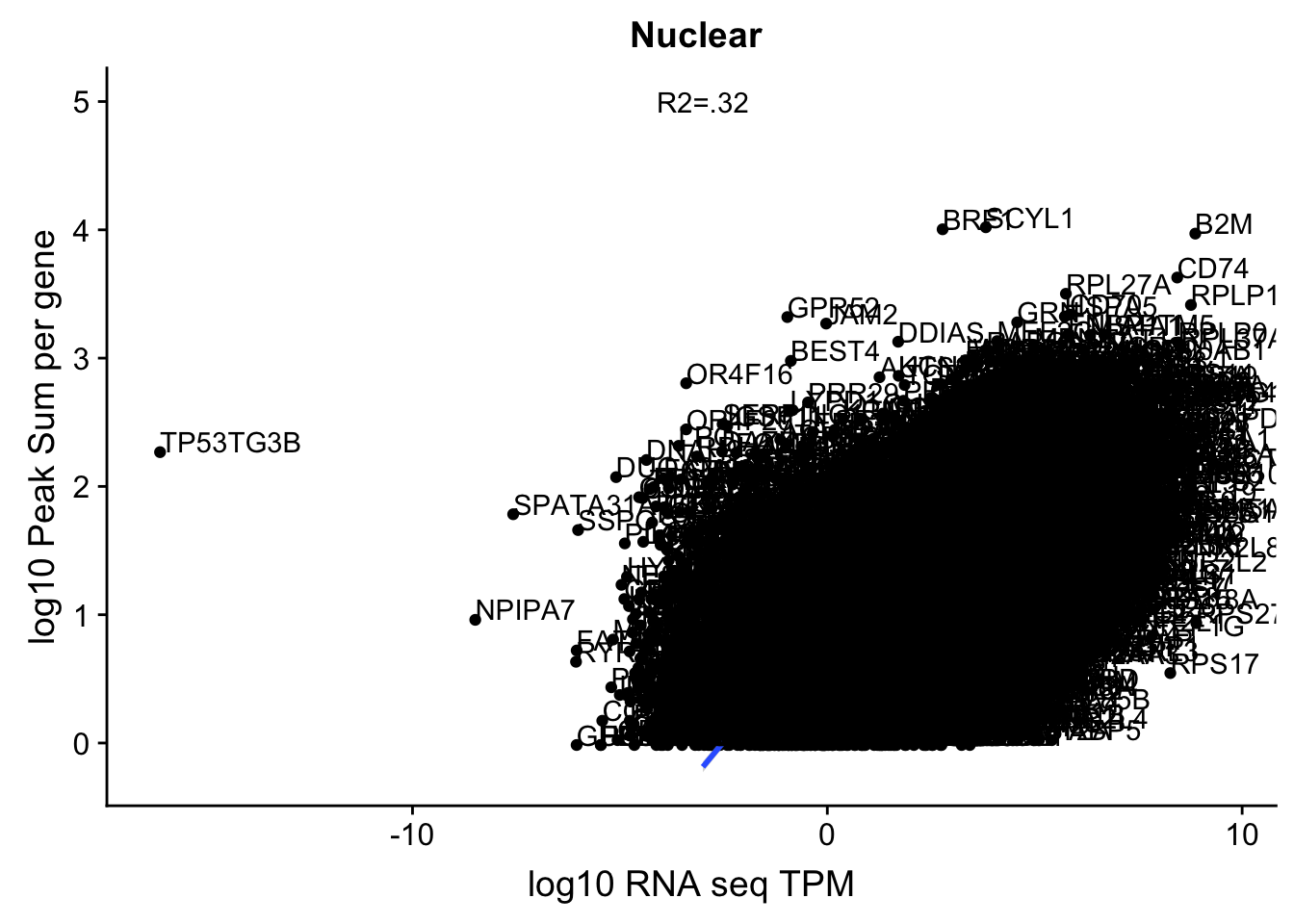
Expand here to see past versions of unnamed-chunk-20-1.png:
| Version | Author | Date |
|---|---|---|
| 6da90e9 | Briana Mittleman | 2018-12-11 |
| afafcc3 | Briana Mittleman | 2018-12-10 |
summary(lm(log10(TPM)~log10(GeneSumNorm),TXN_NormGene_Nuc))
Call:
lm(formula = log10(TPM) ~ log10(GeneSumNorm), data = TXN_NormGene_Nuc)

Residuals:
    Min      1Q  Median      3Q     Max
-8.7166 -0.3526  0.0734  0.4565  3.2783

Coefficients:
                   Estimate Std. Error t value Pr(>|t|)
(Intercept)        -0.13635    0.01665  -8.187 2.95e-16 ***
log10(GeneSumNorm)  0.82341    0.01102  74.727  < 2e-16 ***
---
Signif. codes:  0 '***' 0.001 '**' 0.01 '*' 0.05 '.' 0.1 ' ' 1

Residual standard error: 0.7629 on 11972 degrees of freedom
Multiple R-squared:  0.3181,    Adjusted R-squared:  0.318
F-statistic:  5584 on 1 and 11972 DF,  p-value: < 2.2e-16
title <- ggdraw() + draw_label("Correlation between TPM and 3' Seq \nNA18486", fontface='bold')
plots=plot_grid(corr_18486Tot,corr_18486Nuc)
CorrelationPlot18486=plot_grid(title,plots, ncol=1 , rel_heights = c(.1,1))
ggsave(file="../output/plots/QC_plots/CorrelationWKalisto18486.png",CorrelationPlot18486)Saving 7 x 5 in imageCorrelationPlot18486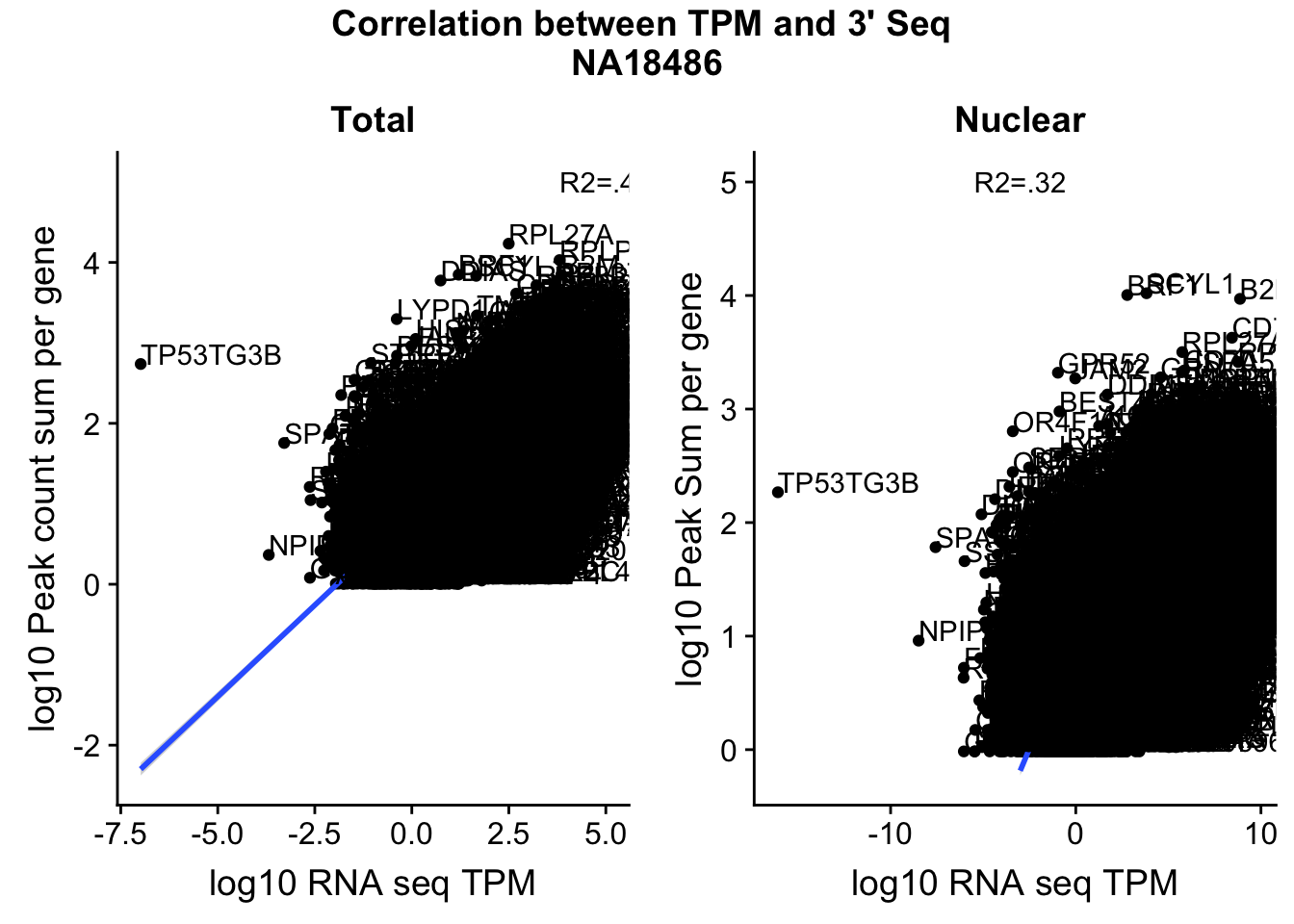
Expand here to see past versions of unnamed-chunk-21-1.png:
| Version | Author | Date |
|---|---|---|
| 6da90e9 | Briana Mittleman | 2018-12-11 |
| 7848485 | Briana Mittleman | 2018-12-07 |
These do not look good. We expect higher correlations. I can make variants of these plots to diagnose the problem.
Just look at the count for the top peak for the gene.
Total:
topPeakCov_total_18486=read.table("../data/PeakCounts/filtered_APApeaks_merged_allchrom_refseqGenes.Transcript_sm_quant.Total_fixed.fc", header=T, stringsAsFactors = F)[,1:7] %>% separate(Geneid, into=c("peak", "chr", "start", "end", "strand", "gene"), sep=":") %>% select(gene, X18486_T) %>% group_by(gene) %>% arrange(gene,desc(X18486_T)) %>% top_n(1)Selecting by X18486_TTXN_TopPeak=TXN_abund %>% inner_join(topPeakCov_total_18486,by="gene")
ggplot(TXN_TopPeak, aes(x=log(TPM+.001), y= log10(X18486_T+.001))) + geom_point() + geom_smooth(aes(x = log10(TPM +.001), y = log10(X18486_T+.001)),method = "lm",se=T) 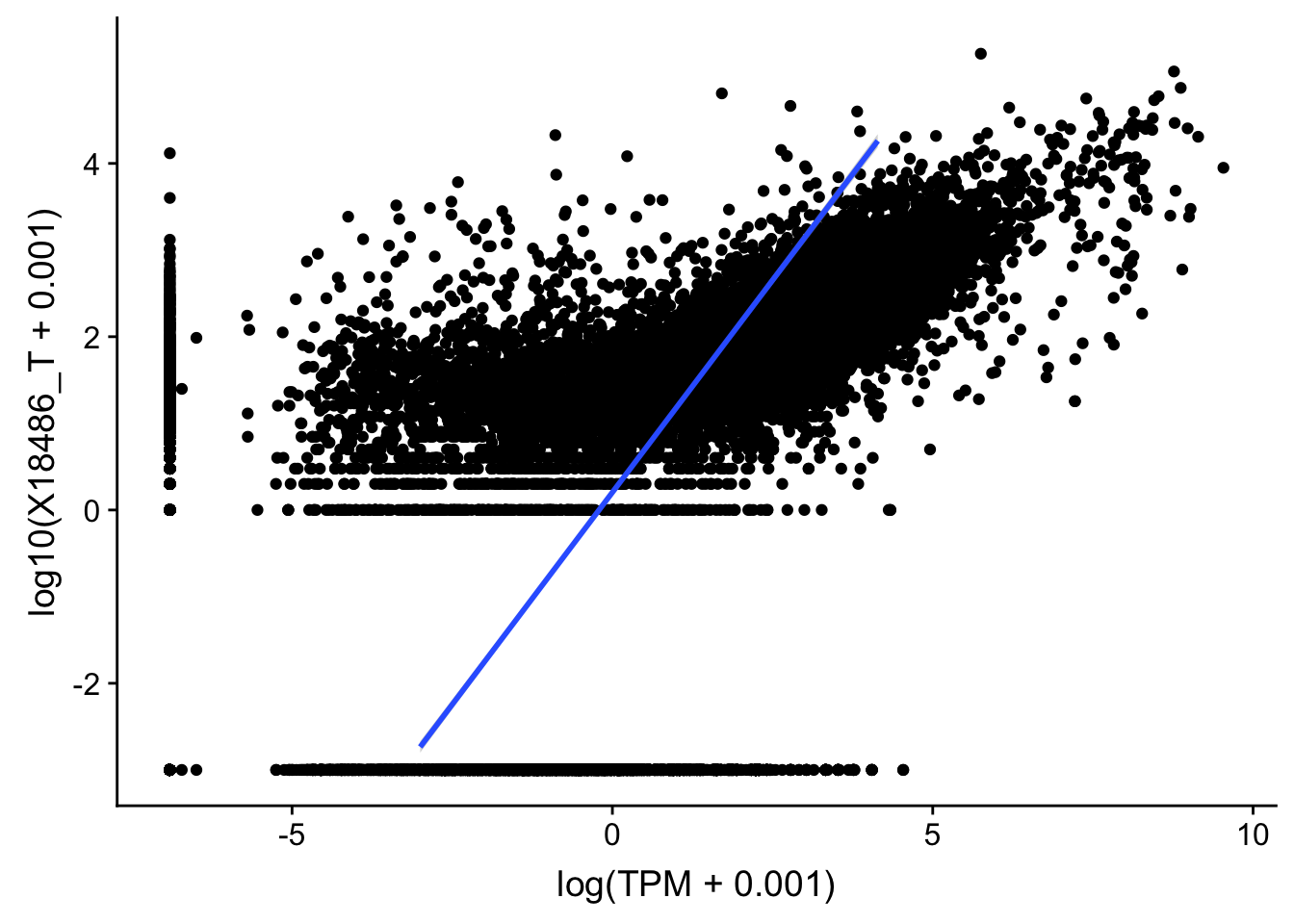
Expand here to see past versions of unnamed-chunk-22-1.png:
| Version | Author | Date |
|---|---|---|
| 6da90e9 | Briana Mittleman | 2018-12-11 |
| daa5818 | Briana Mittleman | 2018-12-07 |
summary(lm(log10(TPM +.001)~log10(X18486_T+ .001),TXN_TopPeak))
Call:
lm(formula = log10(TPM + 0.001) ~ log10(X18486_T + 0.001), data = TXN_TopPeak)

Residuals:
    Min      1Q  Median      3Q     Max
-4.5665 -0.3715  0.3014  0.6793  2.9706

Coefficients:
                        Estimate Std. Error t value Pr(>|t|)
(Intercept)             0.082190   0.008386   9.801   <2e-16 ***
log10(X18486_T + 0.001) 0.360467   0.003491 103.257   <2e-16 ***
---
Signif. codes:  0 '***' 0.001 '**' 0.01 '*' 0.05 '.' 0.1 ' ' 1

Residual standard error: 1.152 on 19537 degrees of freedom
Multiple R-squared:  0.3531,    Adjusted R-squared:  0.353
F-statistic: 1.066e+04 on 1 and 19537 DF,  p-value: < 2.2e-16
Nuclear:
topPeakCov_nuclear_18486=read.table("../data/PeakCounts/filtered_APApeaks_merged_allchrom_refseqGenes.Transcript_sm_quant.Nuclear_fixed.fc", header=T, stringsAsFactors = F)[,1:7] %>% separate(Geneid, into=c("peak", "chr", "start", "end", "strand", "gene"), sep=":") %>% select(gene, X18486_N) %>% group_by(gene) %>% arrange(gene,desc(X18486_N)) %>% top_n(1) Selecting by X18486_NTXN_TopPeak_nuc=TXN_abund %>% inner_join(topPeakCov_nuclear_18486,by="gene")
ggplot(TXN_TopPeak_nuc, aes(x=log(TPM), y= log10(X18486_N))) + geom_point() + geom_smooth(aes(x = log10(TPM), y = log10(X18486_N)),method = "lm",se=T) +xlim(-1,10)Warning: Removed 3349 rows containing non-finite values (stat_smooth).Warning: Removed 2733 rows containing missing values (geom_point).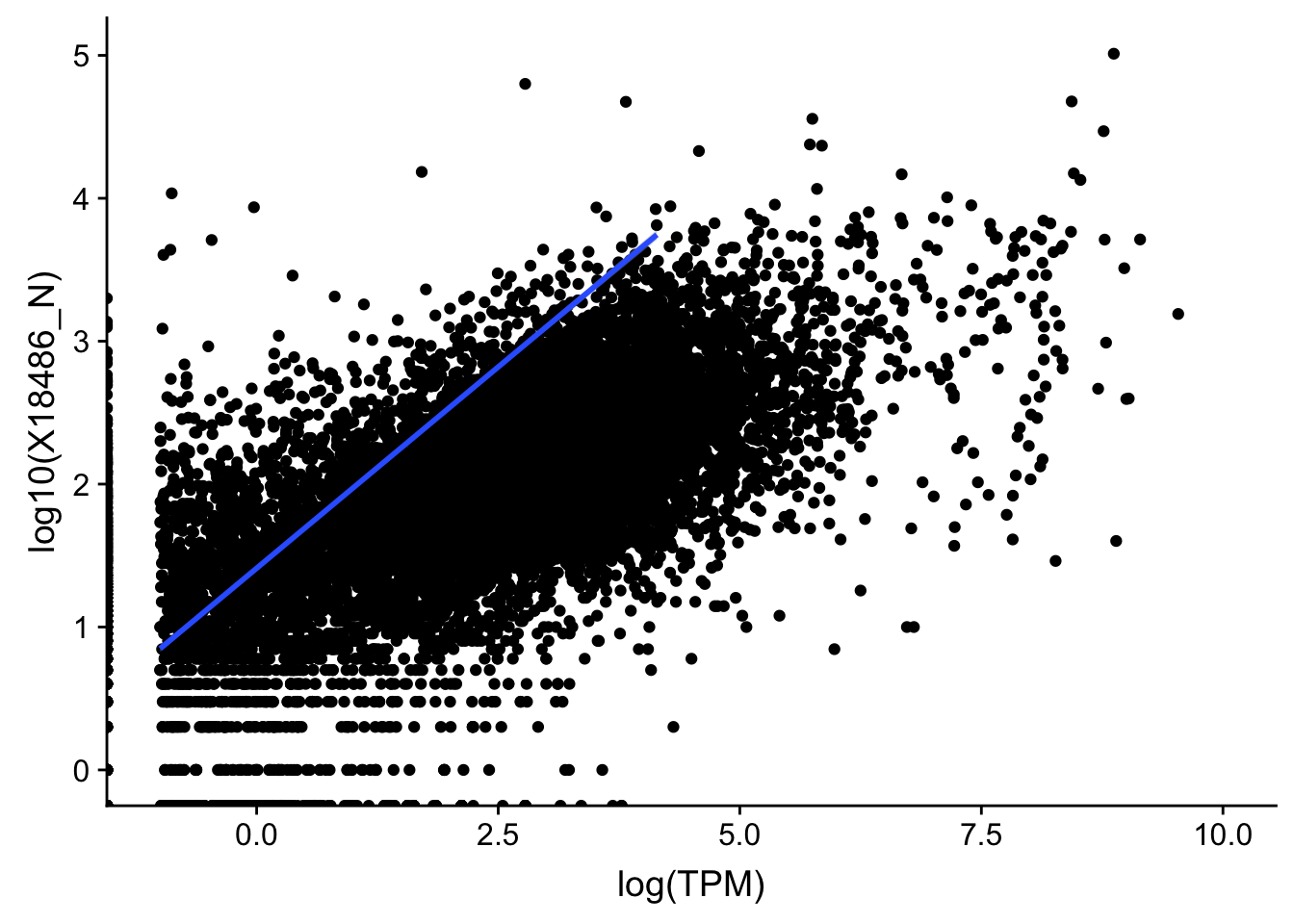
Expand here to see past versions of unnamed-chunk-23-1.png:
| Version | Author | Date |
|---|---|---|
| 6da90e9 | Briana Mittleman | 2018-12-11 |
| daa5818 | Briana Mittleman | 2018-12-07 |
summary(lm(log10(TPM+.001)~log10(X18486_N+.001),TXN_TopPeak_nuc))
Call:
lm(formula = log10(TPM + 0.001) ~ log10(X18486_N + 0.001), data = TXN_TopPeak_nuc)

Residuals:
    Min      1Q  Median      3Q     Max
-4.4195 -0.4383  0.2779  0.6944  3.6667

Coefficients:
                         Estimate Std. Error t value Pr(>|t|)
(Intercept)             -0.385540   0.012683  -30.40   <2e-16 ***
log10(X18486_N + 0.001)  0.546958   0.006061   90.25   <2e-16 ***
---
Signif. codes:  0 '***' 0.001 '**' 0.01 '*' 0.05 '.' 0.1 ' ' 1

Residual standard error: 1.177 on 16302 degrees of freedom
Multiple R-squared:  0.3332,    Adjusted R-squared:  0.3331
F-statistic:  8144 on 1 and 16302 DF,  p-value: < 2.2e-16
Try removing genes with 0 in one the of the columns.
TXN_TopPeak_filt=TXN_TopPeak %>% filter(TPM>0) %>% filter(X18486_T>0)

ggplot(TXN_TopPeak_filt, aes(x=log(TPM), y= log10(X18486_T))) + geom_point() + geom_smooth(aes(x = log10(TPM), y = log10(X18486_T)),method = "lm",se=T)+ geom_text(aes(label=gene),hjust=0, vjust=0)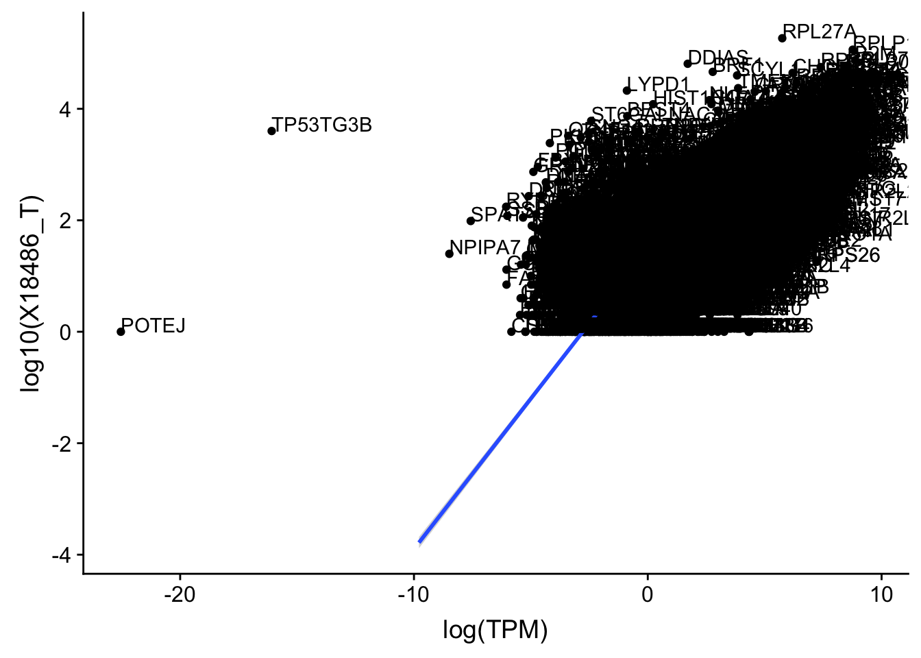
Expand here to see past versions of unnamed-chunk-24-1.png:
| Version | Author | Date |
|---|---|---|
| 6da90e9 | Briana Mittleman | 2018-12-11 |
| daa5818 | Briana Mittleman | 2018-12-07 |
summary(lm(log10(TPM)~log10(X18486_T),TXN_TopPeak_filt))
Call:
lm(formula = log10(TPM) ~ log10(X18486_T), data = TXN_TopPeak_filt)

Residuals:
    Min      1Q  Median      3Q     Max
-9.3583 -0.2584  0.1128  0.4186  2.8988

Coefficients:
                 Estimate Std. Error t value Pr(>|t|)
(Intercept)     -0.906074   0.017369  -52.17   <2e-16 ***
log10(X18486_T)  0.910187   0.008167  111.44   <2e-16 ***
---
Signif. codes:  0 '***' 0.001 '**' 0.01 '*' 0.05 '.' 0.1 ' ' 1

Residual standard error: 0.705 on 12860 degrees of freedom
Multiple R-squared:  0.4913,    Adjusted R-squared:  0.4912
F-statistic: 1.242e+04 on 1 and 12860 DF,  p-value: < 2.2e-16
TXN_TopPeak_filt_nuc=TXN_TopPeak_nuc %>% filter(TPM>0) %>% filter(X18486_N>0)
ggplot(TXN_TopPeak_filt_nuc, aes(x=log(TPM), y= log10(X18486_N))) + geom_point() + geom_smooth(aes(x = log10(TPM), y = log10(X18486_N)),method = "lm",se=T)+ geom_text(aes(label=gene),hjust=0, vjust=0)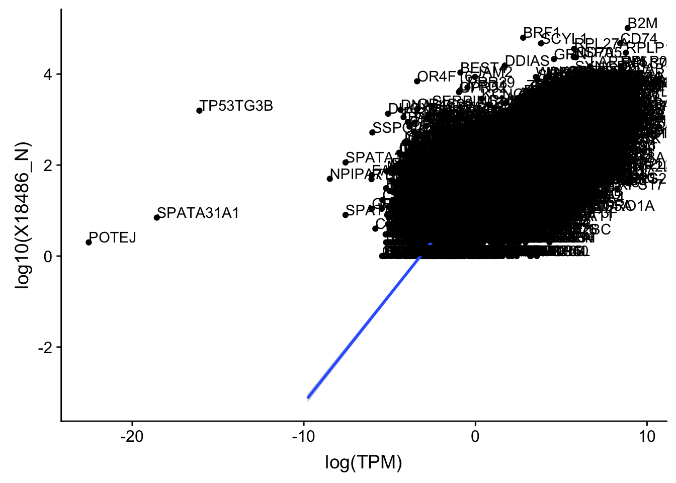
Expand here to see past versions of unnamed-chunk-25-1.png:
| Version | Author | Date |
|---|---|---|
| 6da90e9 | Briana Mittleman | 2018-12-11 |
| daa5818 | Briana Mittleman | 2018-12-07 |
summary(lm(log10(TPM)~log10(X18486_N),TXN_TopPeak_filt_nuc))
Call:
lm(formula = log10(TPM) ~ log10(X18486_N), data = TXN_TopPeak_filt_nuc)

Residuals:
    Min      1Q  Median      3Q     Max
-9.0537 -0.3514  0.0857  0.4783  3.3509

Coefficients:
                 Estimate Std. Error t value Pr(>|t|)
(Intercept)     -1.021815   0.018052   -56.6   <2e-16 ***
log10(X18486_N)  0.957513   0.008878   107.8   <2e-16 ***
---
Signif. codes:  0 '***' 0.001 '**' 0.01 '*' 0.05 '.' 0.1 ' ' 1

Residual standard error: 0.7692 on 13958 degrees of freedom
Multiple R-squared:  0.4545,    Adjusted R-squared:  0.4545
F-statistic: 1.163e+04 on 1 and 13958 DF,  p-value: < 2.2e-16
I should remove these genes because they are outliers:
outlier=c("POTEJ", "SPATA31A1", "TP53TG3B")

TXN_TopPeak_filt2_nuc= TXN_TopPeak_filt_nuc %>% filter(!(gene %in% outlier))

TXN_TopPeak_filt2= TXN_TopPeak_filt %>% filter(!(gene %in% outlier))
Replot:
#nuclear
ggplot(TXN_TopPeak_filt2_nuc, aes(x=log(TPM), y= log10(X18486_N))) + geom_point() + geom_smooth(aes(x = log10(TPM), y = log10(X18486_N)),method = "lm",se=T) 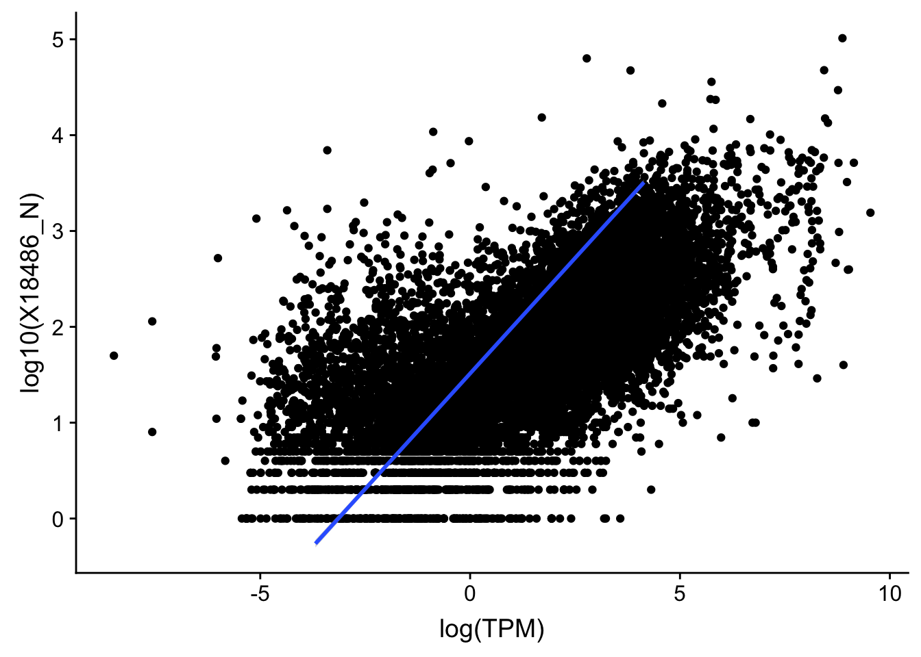
Expand here to see past versions of unnamed-chunk-27-1.png:
| Version | Author | Date |
|---|---|---|
| 6da90e9 | Briana Mittleman | 2018-12-11 |
| daa5818 | Briana Mittleman | 2018-12-07 |
summary(lm(log10(TPM)~log10(X18486_N),TXN_TopPeak_filt2_nuc))
Call:
lm(formula = log10(TPM) ~ log10(X18486_N), data = TXN_TopPeak_filt2_nuc)

Residuals:
    Min      1Q  Median      3Q     Max
-4.2929 -0.3507  0.0844  0.4763  3.3486

Coefficients:
                Estimate Std. Error t value Pr(>|t|)
(Intercept)     -1.01719    0.01781   -57.1   <2e-16 ***
log10(X18486_N)  0.95605    0.00876   109.1   <2e-16 ***
---
Signif. codes:  0 '***' 0.001 '**' 0.01 '*' 0.05 '.' 0.1 ' ' 1

Residual standard error: 0.7588 on 13955 degrees of freedom
Multiple R-squared:  0.4605,    Adjusted R-squared:  0.4604
F-statistic: 1.191e+04 on 1 and 13955 DF,  p-value: < 2.2e-16
#total
ggplot(TXN_TopPeak_filt2, aes(x=log(TPM), y= log10(X18486_T))) + geom_point() + geom_smooth(aes(x = log10(TPM), y = log10(X18486_T)),method = "lm",se=T)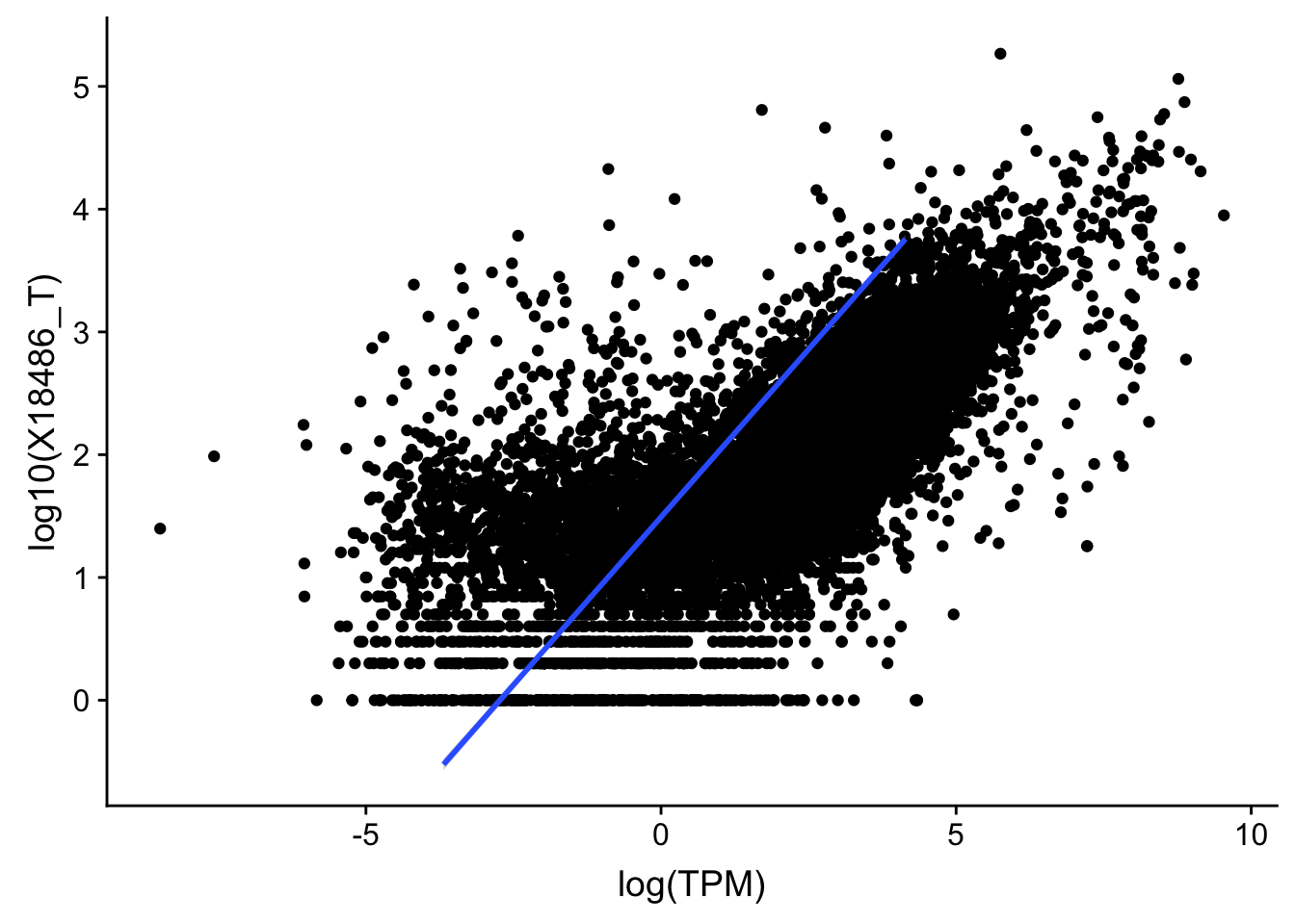
Expand here to see past versions of unnamed-chunk-27-2.png:
| Version | Author | Date |
|---|---|---|
| 6da90e9 | Briana Mittleman | 2018-12-11 |
| daa5818 | Briana Mittleman | 2018-12-07 |
summary(lm(log10(TPM)~log10(X18486_T),TXN_TopPeak_filt))
Call:
lm(formula = log10(TPM) ~ log10(X18486_T), data = TXN_TopPeak_filt)

Residuals:
    Min      1Q  Median      3Q     Max
-9.3583 -0.2584  0.1128  0.4186  2.8988

Coefficients:
                 Estimate Std. Error t value Pr(>|t|)
(Intercept)     -0.906074   0.017369  -52.17   <2e-16 ***
log10(X18486_T)  0.910187   0.008167  111.44   <2e-16 ***
---
Signif. codes:  0 '***' 0.001 '**' 0.01 '*' 0.05 '.' 0.1 ' ' 1

Residual standard error: 0.705 on 12860 degrees of freedom
Multiple R-squared:  0.4913,    Adjusted R-squared:  0.4912
F-statistic: 1.242e+04 on 1 and 12860 DF,  p-value: < 2.2e-16
Genes with 1 peak
Nuclear
First I need to get the genes with just 1 peak.
OnePeak_nuc=read.table("../data/PeakCounts/filtered_APApeaks_merged_allchrom_refseqGenes.Transcript_sm_quant.Nuclear_fixed.fc", header=T, stringsAsFactors = F)[,1:7] %>% separate(Geneid, into=c("peak", "chr", "start", "end", "strand", "gene"), sep=":") %>% group_by(gene) %>% tally() %>% filter(n==1) %>% select(gene)I can join this with the counts to get only the counts for these genes and join with the TXN df.
OnePeak_nuc_cov=read.table("../data/PeakCounts/filtered_APApeaks_merged_allchrom_refseqGenes.Transcript_sm_quant.Nuclear_fixed.fc", header=T, stringsAsFactors = F)[,1:7] %>% separate(Geneid, into=c("peak", "chr", "start", "end", "strand", "gene"), sep=":") %>% select(gene, X18486_N) %>% inner_join(OnePeak_nuc, by="gene") %>% inner_join(TXN_abund, by="gene")Plot and get the correlation:
OnePeak_nuc_cov=OnePeak_nuc_cov %>% filter(TPM>0) %>% filter(X18486_N>0)

ggplot(OnePeak_nuc_cov, aes(x=log10(TPM), y= log10(X18486_N))) + geom_point() + geom_smooth(aes(x = log10(TPM), y = log10(X18486_N)),method = "lm",se=T) + geom_text(aes(label=gene),hjust=0, vjust=0)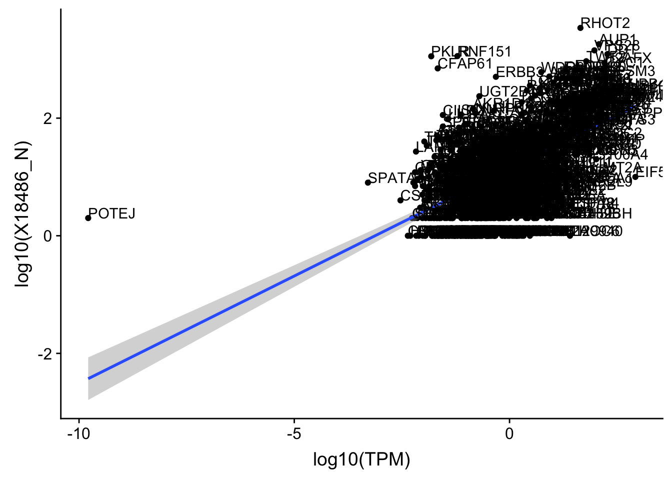
Expand here to see past versions of unnamed-chunk-30-1.png:
| Version | Author | Date |
|---|---|---|
| 6da90e9 | Briana Mittleman | 2018-12-11 |
| 3cd438e | Briana Mittleman | 2018-12-06 |
summary(lm(log10(TPM)~log10(X18486_N),OnePeak_nuc_cov))
Call:
lm(formula = log10(TPM) ~ log10(X18486_N), data = OnePeak_nuc_cov)

Residuals:
    Min      1Q  Median      3Q     Max
-8.8689 -0.5502  0.0730  0.5916  3.2499

Coefficients:
                Estimate Std. Error t value Pr(>|t|)
(Intercept)     -1.17296    0.05663  -20.71   <2e-16 ***
log10(X18486_N)  0.84559    0.04475   18.90   <2e-16 ***
---
Signif. codes:  0 '***' 0.001 '**' 0.01 '*' 0.05 '.' 0.1 ' ' 1

Residual standard error: 0.9359 on 801 degrees of freedom
Multiple R-squared:  0.3084,    Adjusted R-squared:  0.3075
F-statistic: 357.1 on 1 and 801 DF,  p-value: < 2.2e-16
Filter the outlier:
OnePeakN_outlier=c("POTEJ")


OnePeak_nuc_cov_filt= OnePeak_nuc_cov %>% filter(!(gene %in% OnePeakN_outlier))


ggplot(OnePeak_nuc_cov_filt, aes(x=log10(TPM), y= log10(X18486_N))) + geom_point() + geom_smooth(aes(x = log10(TPM), y = log10(X18486_N)),method = "lm",se=T) + geom_text(aes(label=gene),hjust=0, vjust=0)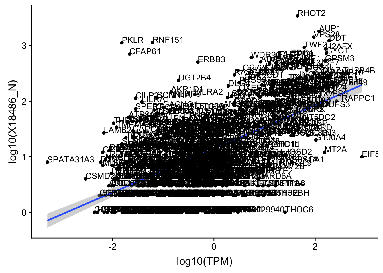
Expand here to see past versions of unnamed-chunk-31-1.png:
| Version | Author | Date |
|---|---|---|
| 6da90e9 | Briana Mittleman | 2018-12-11 |
summary(lm(log10(TPM)~log10(X18486_N),OnePeak_nuc_cov_filt))
Call:
lm(formula = log10(TPM) ~ log10(X18486_N), data = OnePeak_nuc_cov_filt)

Residuals:
    Min      1Q  Median      3Q     Max
-3.2074 -0.5615  0.0608  0.5899  3.2384

Coefficients:
                Estimate Std. Error t value Pr(>|t|)
(Intercept)     -1.14670    0.05345  -21.45   <2e-16 ***
log10(X18486_N)  0.83081    0.04221   19.68   <2e-16 ***
---
Signif. codes:  0 '***' 0.001 '**' 0.01 '*' 0.05 '.' 0.1 ' ' 1

Residual standard error: 0.8823 on 800 degrees of freedom
Multiple R-squared:  0.3263,    Adjusted R-squared:  0.3254
F-statistic: 387.4 on 1 and 800 DF,  p-value: < 2.2e-16
Total
First I need to get the genes with just 1 peak.
OnePeak_tot=read.table("../data/PeakCounts/filtered_APApeaks_merged_allchrom_refseqGenes.Transcript_sm_quant.Total_fixed.fc", header=T, stringsAsFactors = F)[,1:7] %>% separate(Geneid, into=c("peak", "chr", "start", "end", "strand", "gene"), sep=":") %>% group_by(gene) %>% tally() %>% filter(n==1) %>% select(gene)I can join this with the counts to get only the counts for these genes and join with the TXN df.
OnePeak_tot_cov=read.table("../data/PeakCounts/filtered_APApeaks_merged_allchrom_refseqGenes.Transcript_sm_quant.Total_fixed.fc", header=T, stringsAsFactors = F)[,1:7] %>% separate(Geneid, into=c("peak", "chr", "start", "end", "strand", "gene"), sep=":") %>% select(gene, X18486_T) %>% inner_join(OnePeak_tot, by="gene") %>% inner_join(TXN_abund, by="gene")Plot and get the correlation:
OnePeak_tot_cov=OnePeak_tot_cov %>% filter(TPM>0) %>% filter(X18486_T>0)

ggplot(OnePeak_tot_cov, aes(x=log10(TPM), y= log10(X18486_T))) + geom_point() + geom_smooth(aes(x = log10(TPM), y = log10(X18486_T)),method = "lm",se=T) + geom_text(aes(label=gene),hjust=0, vjust=0)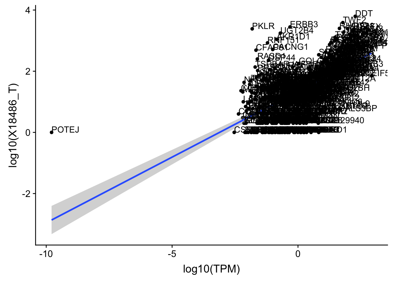
Expand here to see past versions of unnamed-chunk-34-1.png:
| Version | Author | Date |
|---|---|---|
| 6da90e9 | Briana Mittleman | 2018-12-11 |
| 1549daf | Briana Mittleman | 2018-12-07 |
| daa5818 | Briana Mittleman | 2018-12-07 |
summary(lm(log10(TPM)~log10(X18486_T),OnePeak_tot_cov))
Call:
lm(formula = log10(TPM) ~ log10(X18486_T), data = OnePeak_tot_cov)

Residuals:
    Min      1Q  Median      3Q     Max
-8.5586 -0.5457  0.1636  0.6173  2.5539

Coefficients:
                Estimate Std. Error t value Pr(>|t|)
(Intercept)     -1.22867    0.07551  -16.27   <2e-16 ***
log10(X18486_T)  0.86571    0.04861   17.81   <2e-16 ***
---
Signif. codes:  0 '***' 0.001 '**' 0.01 '*' 0.05 '.' 0.1 ' ' 1

Residual standard error: 0.9762 on 536 degrees of freedom
Multiple R-squared:  0.3718,    Adjusted R-squared:  0.3706
F-statistic: 317.2 on 1 and 536 DF,  p-value: < 2.2e-16
Total has the same outlier.
OnePeak_tot_cov_filt= OnePeak_tot_cov %>% filter(!(gene %in% OnePeakN_outlier))


ggplot(OnePeak_tot_cov_filt, aes(x=log10(TPM), y= log10(X18486_T))) + geom_point() + geom_smooth(aes(x = log10(TPM), y = log10(X18486_T)),method = "lm",se=T) + geom_text(aes(label=gene),hjust=0, vjust=0)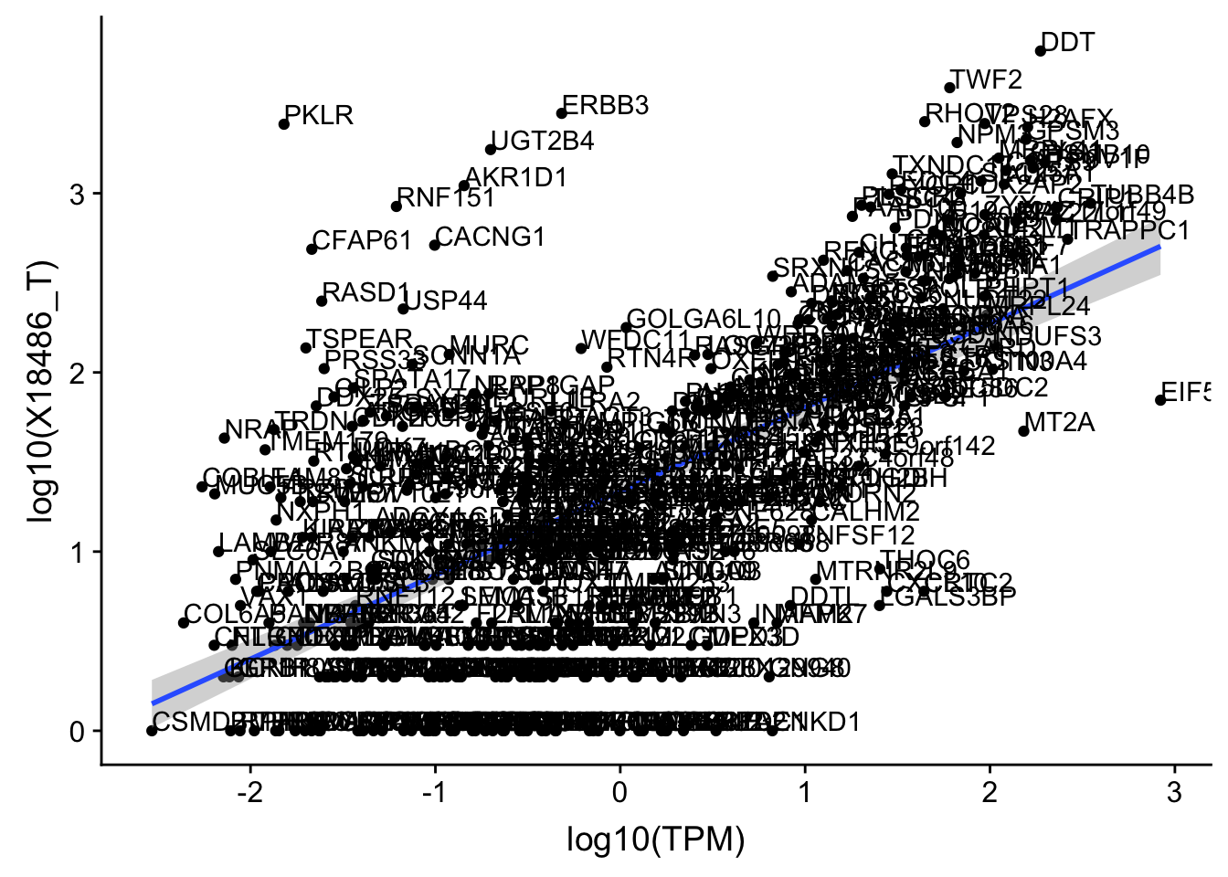
Expand here to see past versions of unnamed-chunk-35-1.png:
| Version | Author | Date |
|---|---|---|
| 6da90e9 | Briana Mittleman | 2018-12-11 |
| afafcc3 | Briana Mittleman | 2018-12-10 |
| 7848485 | Briana Mittleman | 2018-12-07 |
summary(lm(log10(TPM)~log10(X18486_T),OnePeak_tot_cov_filt))
Call:
lm(formula = log10(TPM) ~ log10(X18486_T), data = OnePeak_tot_cov_filt)

Residuals:
    Min      1Q  Median      3Q     Max
-3.4792 -0.5680  0.1435  0.6233  2.5532

Coefficients:
                Estimate Std. Error t value Pr(>|t|)
(Intercept)     -1.17715    0.07013  -16.79   <2e-16 ***
log10(X18486_T)  0.83818    0.04510   18.59   <2e-16 ***
---
Signif. codes:  0 '***' 0.001 '**' 0.01 '*' 0.05 '.' 0.1 ' ' 1

Residual standard error: 0.9039 on 535 degrees of freedom
Multiple R-squared:  0.3923,    Adjusted R-squared:  0.3912
F-statistic: 345.4 on 1 and 535 DF,  p-value: < 2.2e-16
I want to visualize some of these outliers.
These dont look great, I am continuing this section of the analysis by looking at the Peak to gene assignment
Q: For each gene, what percentage of reads assigned fall within 1, 2, 3, etc… peaks, we would expect that for many genes >90% of the reads fall within 1 peak, for a few 2 peaks, etc…?
Plot: Y-axis: Number of genes, X-axis: how many peaks is needed to “capture” 90%, 80%, … 50% of the reads assigned to that gene (using different colors).
Start with analysis to see how many peaks are needed to capture 90% of the reads assigned to the gene. I will start by looking at the number of reads that map to peaks in genes. To do this I can group on genes in the peak coverage and get the sum.
nuclear_covBygene=read.table("../data/PeakCounts/filtered_APApeaks_merged_allchrom_refseqGenes.Transcript_sm_quant.Nuclear_fixed.fc", header=T, stringsAsFactors = F)[,1:7] %>% separate(Geneid, into=c("peak", "chr", "start", "end", "strand", "gene"), sep=":") %>% select(gene, X18486_N) %>% group_by(gene) %>% summarize(GeneSum=sum(X18486_N)) %>% mutate(per90=GeneSum*.9)%>% mutate(per80=GeneSum*.8)%>% mutate(per70=GeneSum*.7)%>% mutate(per60=GeneSum*.6)%>% mutate(per50=GeneSum*.5)
total_covBygene=read.table("../data/PeakCounts/filtered_APApeaks_merged_allchrom_refseqGenes.Transcript_sm_quant.Total_fixed.fc", header=T, stringsAsFactors = F)[,1:7] %>% separate(Geneid, into=c("peak", "chr", "start", "end", "strand", "gene"), sep=":") %>% select(gene, X18486_T) %>% group_by(gene) %>% summarize(GeneSum=sum(X18486_T))%>% mutate(per90=GeneSum*.9)%>% mutate(per80=GeneSum*.8)%>% mutate(per70=GeneSum*.7)%>% mutate(per60=GeneSum*.6)%>% mutate(per50=GeneSum*.5)
Write these out to use them in the script:
write.table(file="../data/UnderstandPeaksQC/Nuclear_PerCovbyGene.txt", nuclear_covBygene, quote=F, col.names = T, row.names = F)
write.table(file="../data/UnderstandPeaksQC/Total_PerCovbyGene.txt", total_covBygene, quote=F, col.names = T,row.names = F)
Try in R
#groupedNuclear=sumforeachgene %>% sort(ind) %>% cumulativesum %>% dividebygenesum %>% filter(only90) %>% count()
#remove genes with 0 count sum

nuclear_90Cov=read.table("../data/PeakCounts/filtered_APApeaks_merged_allchrom_refseqGenes.Transcript_sm_quant.Nuclear_fixed.fc", header=T, stringsAsFactors = F)[,1:7] %>% separate(Geneid, into=c("peak", "chr", "start", "end", "strand", "gene"), sep=":") %>% select(gene, X18486_N) %>% group_by(gene) %>%  arrange(gene,desc(X18486_N)) %>%  mutate(SUM = cumsum(X18486_N)) %>% full_join(nuclear_covBygene,by="gene") %>% filter(GeneSum >0) %>% mutate(perSum=SUM/GeneSum) %>% mutate(perSum_lag=lag(perSum,1)) %>%  replace_na(list(perSum_lag =0)) %>% filter(perSum_lag<.9) %>% tally() %>% rename("90"=n)

nuclear_80Cov=read.table("../data/PeakCounts/filtered_APApeaks_merged_allchrom_refseqGenes.Transcript_sm_quant.Nuclear_fixed.fc", header=T, stringsAsFactors = F)[,1:7] %>% separate(Geneid, into=c("peak", "chr", "start", "end", "strand", "gene"), sep=":") %>% select(gene, X18486_N) %>% group_by(gene) %>%  arrange(gene,desc(X18486_N)) %>%  mutate(SUM = cumsum(X18486_N)) %>% full_join(nuclear_covBygene,by="gene") %>% filter(GeneSum >0) %>% mutate(perSum=SUM/GeneSum) %>% mutate(perSum_lag=lag(perSum,1)) %>%  replace_na(list(perSum_lag =0)) %>% filter(perSum_lag<.8) %>% tally() %>% rename("80"=n)

nuclear_70Cov=read.table("../data/PeakCounts/filtered_APApeaks_merged_allchrom_refseqGenes.Transcript_sm_quant.Nuclear_fixed.fc", header=T, stringsAsFactors = F)[,1:7] %>% separate(Geneid, into=c("peak", "chr", "start", "end", "strand", "gene"), sep=":") %>% select(gene, X18486_N) %>% group_by(gene) %>%  arrange(gene,desc(X18486_N)) %>%  mutate(SUM = cumsum(X18486_N)) %>% full_join(nuclear_covBygene,by="gene") %>% filter(GeneSum >0) %>% mutate(perSum=SUM/GeneSum) %>% mutate(perSum_lag=lag(perSum,1)) %>%  replace_na(list(perSum_lag =0)) %>% filter(perSum_lag<.7) %>% tally() %>% rename("70"=n)

nuclear_60Cov=read.table("../data/PeakCounts/filtered_APApeaks_merged_allchrom_refseqGenes.Transcript_sm_quant.Nuclear_fixed.fc", header=T, stringsAsFactors = F)[,1:7] %>% separate(Geneid, into=c("peak", "chr", "start", "end", "strand", "gene"), sep=":") %>% select(gene, X18486_N) %>% group_by(gene) %>%  arrange(gene,desc(X18486_N)) %>%  mutate(SUM = cumsum(X18486_N)) %>% full_join(nuclear_covBygene,by="gene") %>% filter(GeneSum >0) %>% mutate(perSum=SUM/GeneSum) %>% mutate(perSum_lag=lag(perSum,1)) %>%  replace_na(list(perSum_lag =0)) %>% filter(perSum_lag<.6) %>% tally() %>% rename("60"=n)

nuclear_50Cov=read.table("../data/PeakCounts/filtered_APApeaks_merged_allchrom_refseqGenes.Transcript_sm_quant.Nuclear_fixed.fc", header=T, stringsAsFactors = F)[,1:7] %>% separate(Geneid, into=c("peak", "chr", "start", "end", "strand", "gene"), sep=":") %>% select(gene, X18486_N) %>% group_by(gene) %>%  arrange(gene,desc(X18486_N)) %>%  mutate(SUM = cumsum(X18486_N)) %>% full_join(nuclear_covBygene,by="gene") %>% filter(GeneSum >0) %>% mutate(perSum=SUM/GeneSum) %>% mutate(perSum_lag=lag(perSum,1)) %>%  replace_na(list(perSum_lag =0)) %>% filter(perSum_lag<.5) %>% tally() %>% rename("50"=n)
Join these to plot them:
nuclear_PercentPeakCov= nuclear_90Cov %>% left_join(nuclear_80Cov, by="gene") %>% left_join(nuclear_70Cov, by="gene") %>% left_join(nuclear_60Cov, by="gene") %>% left_join(nuclear_50Cov, by="gene")

nuclear_PercentPeakCov_melt=melt(nuclear_PercentPeakCov,id.vars = "gene")
nucPeakCov=ggplot(nuclear_PercentPeakCov_melt, aes(x=value,fill=variable))+ geom_histogram(position="dodge", bins=30) + labs(y="Number of Genes", x="Number of Peaks", title="Nuclear: Number of Peaks to capture % of Gene count") + facet_grid(~variable) + xlim(0,30)
nucPeakCov_cdf=ggplot(nuclear_PercentPeakCov_melt, aes(x=value,col=variable))+ stat_ecdf(geom="step")+ labs(y="Percent of Genes", x="Number of Peaks", title="Nuclear: Number of Peaks to capture % of Gene count") + scale_x_continuous(breaks=seq(1,30,2),limits=c(0,30))
ggplot(nuclear_PercentPeakCov_melt, aes(x=value,fill=variable, by=variable))+ geom_density(alpha=.4) + labs(y="Number of Genes", x="Number of Peaks", title="Nuclear: Number of Peaks to capture % of Gene count")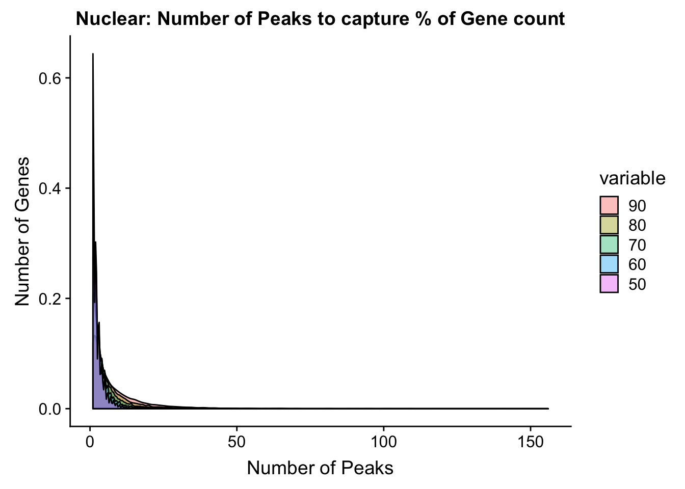
Expand here to see past versions of unnamed-chunk-40-1.png:
| Version | Author | Date |
|---|---|---|
| 6da90e9 | Briana Mittleman | 2018-12-11 |
Try this with total:
total_90Cov=read.table("../data/PeakCounts/filtered_APApeaks_merged_allchrom_refseqGenes.Transcript_sm_quant.Total_fixed.fc", header=T, stringsAsFactors = F)[,1:7] %>% separate(Geneid, into=c("peak", "chr", "start", "end", "strand", "gene"), sep=":") %>% select(gene, X18486_T) %>% group_by(gene) %>%  arrange(gene,desc(X18486_T)) %>%  mutate(SUM = cumsum(X18486_T)) %>% full_join(total_covBygene,by="gene") %>% filter(GeneSum >0) %>% mutate(perSum=SUM/GeneSum) %>% mutate(perSum_lag=lag(perSum,1)) %>%  replace_na(list(perSum_lag =0)) %>% filter(perSum_lag<.9) %>% tally() %>% rename("90"=n)

total_80Cov=read.table("../data/PeakCounts/filtered_APApeaks_merged_allchrom_refseqGenes.Transcript_sm_quant.Total_fixed.fc", header=T, stringsAsFactors = F)[,1:7] %>% separate(Geneid, into=c("peak", "chr", "start", "end", "strand", "gene"), sep=":") %>% select(gene, X18486_T) %>% group_by(gene) %>%  arrange(gene,desc(X18486_T)) %>%  mutate(SUM = cumsum(X18486_T)) %>% full_join(total_covBygene,by="gene") %>% filter(GeneSum >0) %>% mutate(perSum=SUM/GeneSum) %>% mutate(perSum_lag=lag(perSum,1)) %>%  replace_na(list(perSum_lag =0)) %>% filter(perSum_lag<.8) %>% tally() %>% rename("80"=n)

total_70Cov=read.table("../data/PeakCounts/filtered_APApeaks_merged_allchrom_refseqGenes.Transcript_sm_quant.Total_fixed.fc", header=T, stringsAsFactors = F)[,1:7] %>% separate(Geneid, into=c("peak", "chr", "start", "end", "strand", "gene"), sep=":") %>% select(gene, X18486_T) %>% group_by(gene) %>%  arrange(gene,desc(X18486_T)) %>%  mutate(SUM = cumsum(X18486_T)) %>% full_join(total_covBygene,by="gene") %>% filter(GeneSum >0) %>% mutate(perSum=SUM/GeneSum) %>% mutate(perSum_lag=lag(perSum,1)) %>%  replace_na(list(perSum_lag =0)) %>% filter(perSum_lag<.7) %>% tally() %>% rename("70"=n)

total_60Cov=read.table("../data/PeakCounts/filtered_APApeaks_merged_allchrom_refseqGenes.Transcript_sm_quant.Total_fixed.fc", header=T, stringsAsFactors = F)[,1:7] %>% separate(Geneid, into=c("peak", "chr", "start", "end", "strand", "gene"), sep=":") %>% select(gene, X18486_T) %>% group_by(gene) %>%  arrange(gene,desc(X18486_T)) %>%  mutate(SUM = cumsum(X18486_T)) %>% full_join(total_covBygene,by="gene") %>% filter(GeneSum >0) %>% mutate(perSum=SUM/GeneSum) %>% mutate(perSum_lag=lag(perSum,1)) %>%  replace_na(list(perSum_lag =0)) %>% filter(perSum_lag<.6) %>% tally() %>% rename("60"=n)

total_50Cov=read.table("../data/PeakCounts/filtered_APApeaks_merged_allchrom_refseqGenes.Transcript_sm_quant.Total_fixed.fc", header=T, stringsAsFactors = F)[,1:7] %>% separate(Geneid, into=c("peak", "chr", "start", "end", "strand", "gene"), sep=":") %>% select(gene, X18486_T) %>% group_by(gene) %>%  arrange(gene,desc(X18486_T)) %>%  mutate(SUM = cumsum(X18486_T)) %>% full_join(total_covBygene,by="gene") %>% filter(GeneSum >0) %>% mutate(perSum=SUM/GeneSum) %>% mutate(perSum_lag=lag(perSum,1)) %>%  replace_na(list(perSum_lag =0)) %>% filter(perSum_lag<.5) %>% tally() %>% rename("50"=n)
Put together:
total_PercentPeakCov= total_90Cov %>% left_join(total_80Cov, by="gene") %>% left_join(total_70Cov, by="gene") %>% left_join(total_60Cov, by="gene") %>% left_join(total_50Cov, by="gene")

total_PercentPeakCov_melt=melt(total_PercentPeakCov,id.vars = "gene")
totPeakCov=ggplot(total_PercentPeakCov_melt, aes(x=value,fill=variable))+ geom_histogram(position="dodge", bins=30) + labs(y="Number of Genes", x="Number of Peaks", title="Total: Number of Peaks to capture % of Gene count") + facet_grid(~variable) + xlim(0,30)
totPeakCov_cdf=ggplot(total_PercentPeakCov_melt, aes(x=value,col=variable))+ stat_ecdf(geom="step")+ labs(y="Percent of Genes", x="Number of Peaks", title="Total: Number of Peaks to capture % of Gene count") + scale_x_continuous(breaks=seq(1,30,2),limits=c(0,30))
ggplot(total_PercentPeakCov_melt, aes(x=value,fill=variable, by=variable))+ geom_density(alpha=.4) + labs(y="Number of Genes", x="Number of Peaks", title="Nuclear: Number of Peaks to capture % of Gene count")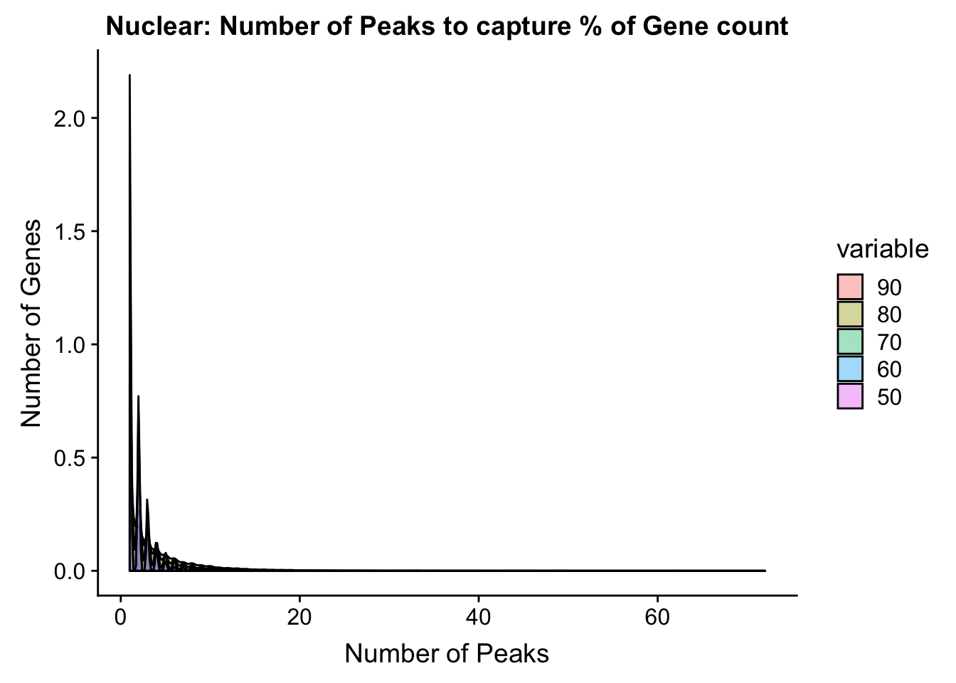
Expand here to see past versions of unnamed-chunk-43-1.png:
| Version | Author | Date |
|---|---|---|
| 6da90e9 | Briana Mittleman | 2018-12-11 |
| 1549daf | Briana Mittleman | 2018-12-07 |
| daa5818 | Briana Mittleman | 2018-12-07 |
PeakCovPerGeneCount=plot_grid(totPeakCov,nucPeakCov, ncol = 1)Warning: Removed 85 rows containing non-finite values (stat_bin).Warning: Removed 810 rows containing non-finite values (stat_bin).ggsave(file="../output/plots/QC_plots/PeakCovPerGeneCount.png",PeakCovPerGeneCount)Saving 7 x 5 in imagePeakCovPerGeneCountCDF=plot_grid(totPeakCov_cdf,nucPeakCov_cdf,ncol=1)Warning: Removed 85 rows containing non-finite values (stat_ecdf).Warning: Removed 810 rows containing non-finite values (stat_ecdf).ggsave(file="../output/plots/QC_plots/PeakCovPerGeneCountCDF.png",PeakCovPerGeneCountCDF)Saving 7 x 5 in imageThese look good. We could use this to filter. I would compute the percent of the gene each peak covers in each individual then I could filter peaks that cover
I need to separate the libraries by line and fraction.
fc_peaks=fc_peaks %>% separate(Status, into=c("line", "fraction"), sep="_") %>% mutate(PerReadPeak=Assigned/(Assigned+Unassigned_NoFeatures))This number is the reads assigned to peaks out of all reads mapping to genome.
I can now melt these data by line and fraction
fc_peaks_melt=melt(fc_peaks, id.vars = c("line", "fraction"))Warning: attributes are not identical across measure variables; they will
be droppedfc_peaks_melt_PerRead=fc_peaks_melt %>% filter(variable=="PerReadPeak")
fc_peaks_melt_PerRead$value=as.numeric(fc_peaks_melt_PerRead$value)ggplot(fc_peaks_melt_PerRead,aes( x=line, y=value, by=fraction, fill=fraction))+ geom_col(pos="dodge") +theme(axis.text.x = element_text(angle = 90, hjust = 1),axis.text.y = element_text(size=12),axis.title.y=element_text(size=10,face="bold"), axis.title.x=element_text(size=12,face="bold"))+ scale_fill_manual(values=c("deepskyblue3","darkviolet")) + labs(title="Percent of reads mapping to peaks by line and fraction", y="Reads mapping to peaks/all mapping reads")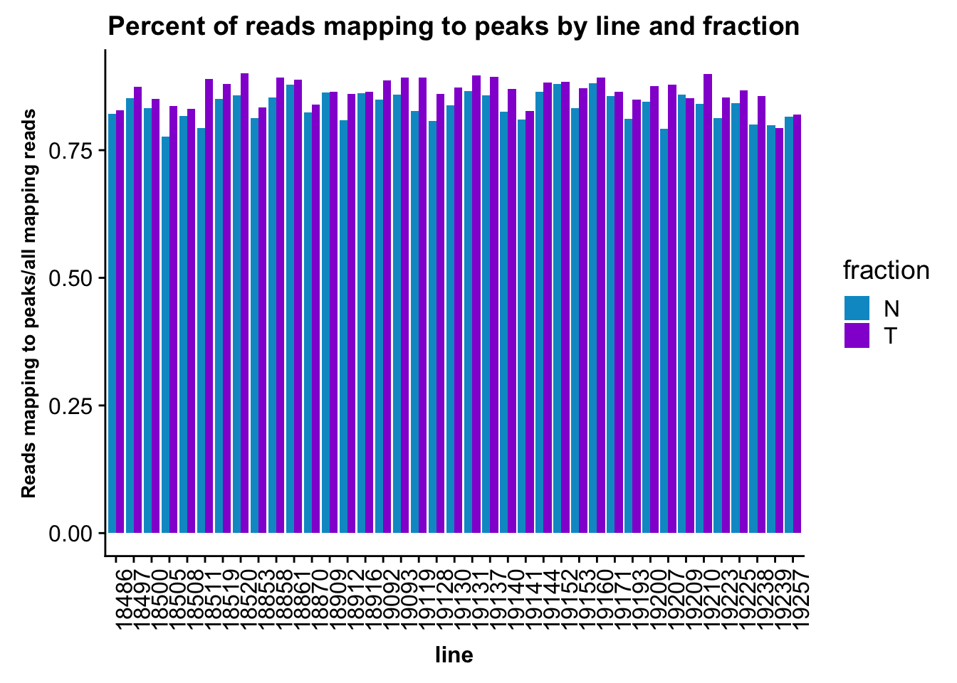
Expand here to see past versions of unnamed-chunk-49-1.png:
| Version | Author | Date |
|---|---|---|
| 6da90e9 | Briana Mittleman | 2018-12-11 |
It may be more interesting to look at this by fraction, with error bars.
fc_peaks_melt_PerRead_byfrac= fc_peaks_melt_PerRead %>% group_by(fraction) %>% summarise(mean=mean(value), sd=sd(value))Plot this:
ggplot(fc_peaks_melt_PerRead_byfrac,aes(x=fraction, y=mean, fill=fraction)) + geom_col()+ geom_errorbar(aes(ymin=mean-sd, ymax=mean+sd), width=.2)+ theme(axis.text.y = element_text(size=12),axis.title.y=element_text(size=10,face="bold"), axis.title.x=element_text(size=12,face="bold"))+ scale_fill_manual(values=c("deepskyblue3","darkviolet"))+ labs(title="Percent of reads mapping to peaks by fraction", y="Reads mapping to peaks/all mapping reads")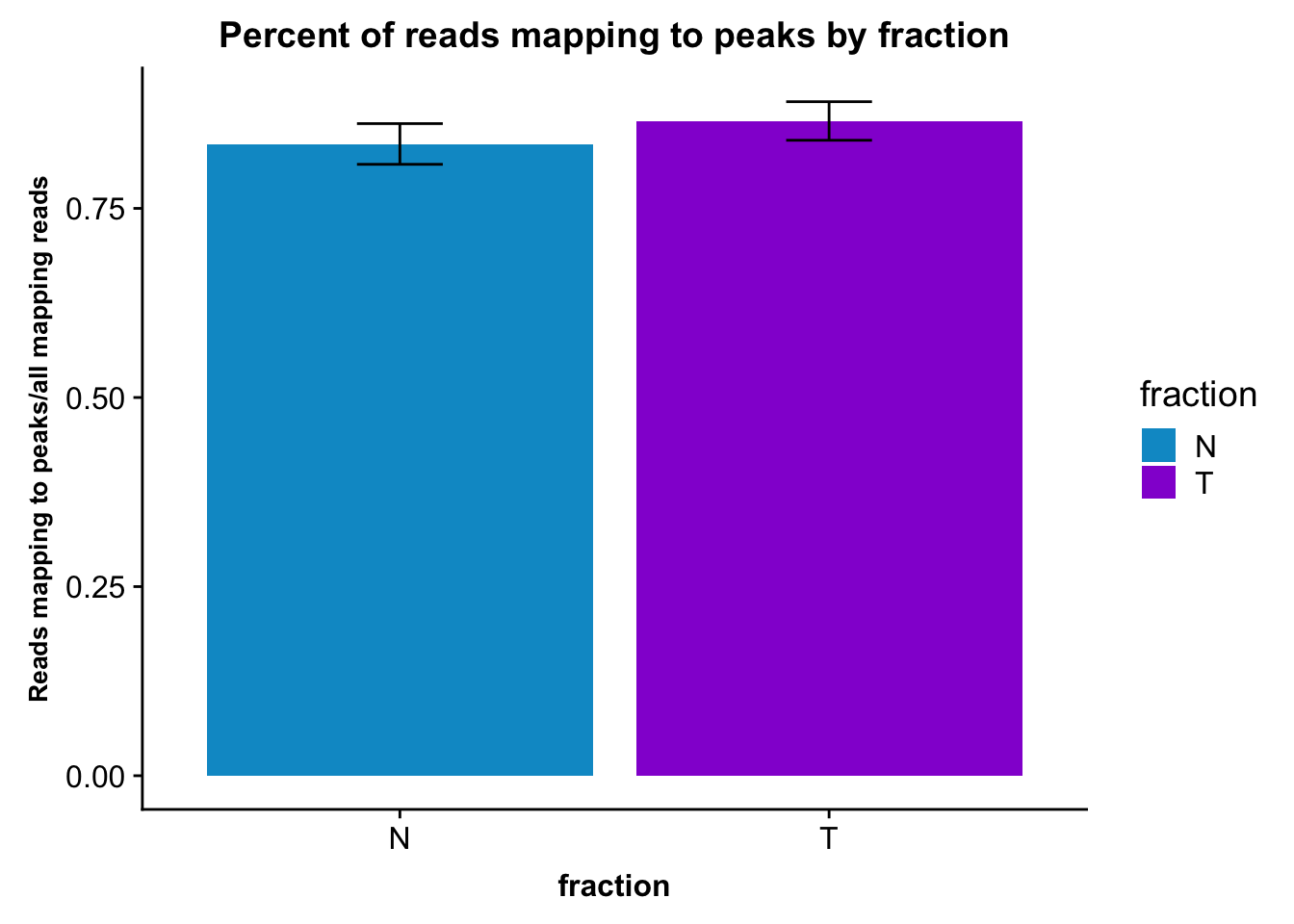
Expand here to see past versions of unnamed-chunk-51-1.png:
| Version | Author | Date |
|---|---|---|
| 6da90e9 | Briana Mittleman | 2018-12-11 |
Now I want to look at how many reads map to gene. I will use the transcript annotations that I used for the peaks.
- /project2/gilad/briana/genome_anotation_data/ncbiRefSeq_sm_noChr.sort.mRNA.bed
I need to make this an SAF file.
* GeneID * Chr * Start * End * Strand
RefSeqmRNA2SAF.py
#python
from misc_helper import *
fout = file("/project2/gilad/briana/genome_anotation_data/ncbiRefSeq_sm_noChr.sort.mRNA.SAF","w")
fout.write("GeneID\tChr\tStart\tEnd\tStrand\n")
for ln in open("/project2/gilad/briana/genome_anotation_data/ncbiRefSeq_sm_noChr.sort.mRNA.bed"):
    chrom, start, end, gene, score, strand = ln.split()
    start_i=int(start)
    end_i=int(end)
    fout.write("%s\t%s\t%d\t%d\t%s\n"%(gene, chrom, start_i, end_i, strand))
fout.close()
ref_geneTranscript_fc.sh
#!/bin/bash

#SBATCH --job-name=ref_geneTranscript_fc
#SBATCH --account=pi-yangili1
#SBATCH --time=24:00:00
#SBATCH --output=ref_geneTranscript_fc.out
#SBATCH --error=ref_geneTranscript_fc.err
#SBATCH --partition=broadwl
#SBATCH --mem=12G
#SBATCH --mail-type=END


module load Anaconda3
source activate three-prime-env

featureCounts -O -a /project2/gilad/briana/genome_anotation_data/ncbiRefSeq_sm_noChr.sort.mRNA.SAF -F SAF -o /project2/gilad/briana/threeprimeseq/data/UnderstandPeaksQC/RefSeqTranscript_AllLibraries.fc /project2/gilad/briana/threeprimeseq/data/sort/*sort.bam -s 2
fix_Genefc_summary.py
infile= open("/Users/bmittleman1/Documents/Gilad_lab/threeprimeseq/data/UnderstandPeaksQC/RefSeqTranscript_AllLibraries.fc.summary", "r")
fout = open("/Users/bmittleman1/Documents/Gilad_lab/threeprimeseq/data/UnderstandPeaksQC/RefSeqTranscript_AllLibraries.fc.summary_fixed",'w')
for line, i in enumerate(infile):
    if line == 0:
        i_list=i.split()
        libraries=[i_list[0]]
        for sample in i_list[1:]:
            full = sample.split("/")[7]
            samp= full.split("-")[2:4]
            lim="_"
            samp_st=lim.join(samp)
            libraries.append(samp_st)
        print(libraries)
        first_line= "\t".join(libraries)
        fout.write(first_line + '\n' )
    else:
        fout.write(i)
fout.close()
fc_gene_peaks=read.table("../data/UnderstandPeaksQC/RefSeqTranscript_AllLibraries.fc.summary_fixed", stringsAsFactors = F) %>% t()
fc_gene_peaks=as.data.frame(fc_gene_peaks)
colnames(fc_gene_peaks)=as.character(unlist(fc_gene_peaks[1,]))
fc_gene_peaks=fc_gene_peaks[-1,]
fc_gene_peaks$Assigned=as.numeric(as.character(fc_gene_peaks$Assigned))
fc_gene_peaks$Unassigned_NoFeatures=as.numeric(as.character(fc_gene_peaks$Unassigned_NoFeatures))I need to separate the libraries by line and fraction.
fc_gene_peaks=fc_gene_peaks %>% separate(Status, into=c("line", "fraction"), sep="_") %>% mutate(PerReadPeak=Assigned/(Assigned+Unassigned_NoFeatures))Melt this:
fc_gene_peaks_melt=melt(fc_gene_peaks, id.vars = c("line", "fraction"))Warning: attributes are not identical across measure variables; they will
be droppedfc_gene_peaks_PerRead=fc_gene_peaks_melt %>% filter(variable=="PerReadPeak")
fc_gene_peaks_PerRead$value=as.numeric(fc_gene_peaks_PerRead$value)GGplot:
ggplot(fc_gene_peaks_PerRead,aes( x=line, y=value, by=fraction, fill=fraction))+ geom_col(pos="dodge") +theme(axis.text.x = element_text(angle = 90, hjust = 1),axis.text.y = element_text(size=12),axis.title.y=element_text(size=10,face="bold"), axis.title.x=element_text(size=12,face="bold"))+ scale_fill_manual(values=c("deepskyblue3","darkviolet")) + labs(title="Percent of reads mapping to Transcripts by line and fraction", y="Reads mapping to transcripts/all mapping reads")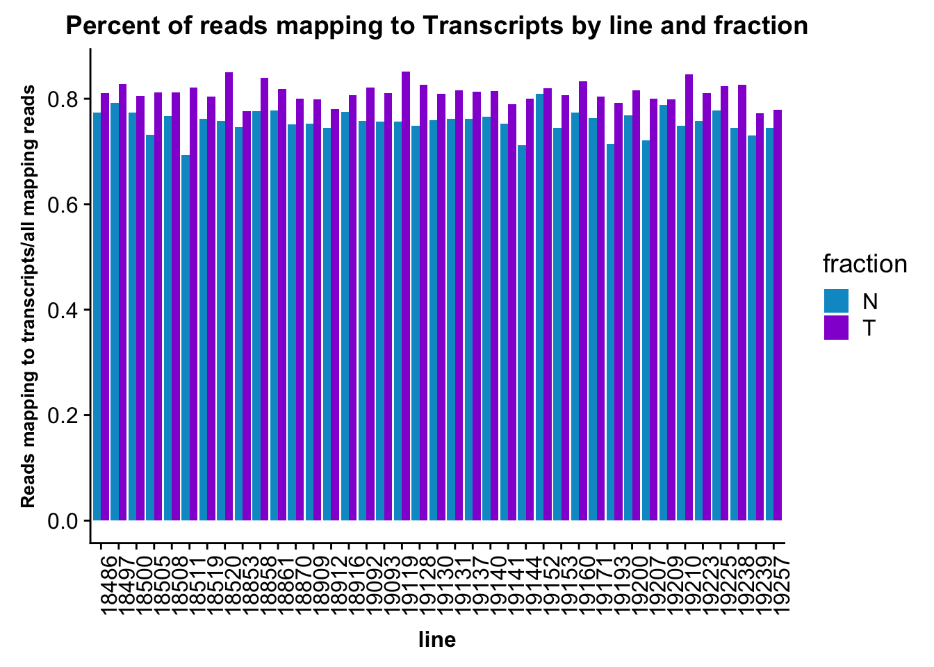
Expand here to see past versions of unnamed-chunk-58-1.png:
| Version | Author | Date |
|---|---|---|
| 6da90e9 | Briana Mittleman | 2018-12-11 |
Do this by fraction.
fc_gene_peaks_PerRead_byfrac= fc_gene_peaks_PerRead %>% group_by(fraction) %>% summarise(mean=mean(value), sd=sd(value))Plot this:
ggplot(fc_gene_peaks_PerRead_byfrac,aes(x=fraction, y=mean, fill=fraction)) + geom_col()+ geom_errorbar(aes(ymin=mean-sd, ymax=mean+sd), width=.2)+ theme(axis.text.y = element_text(size=12),axis.title.y=element_text(size=10,face="bold"), axis.title.x=element_text(size=12,face="bold"))+ scale_fill_manual(values=c("deepskyblue3","darkviolet"))+ labs(title="Percent of reads mapping to Transcripts by fraction", y="Reads mapping to Transcripts/all mapping reads")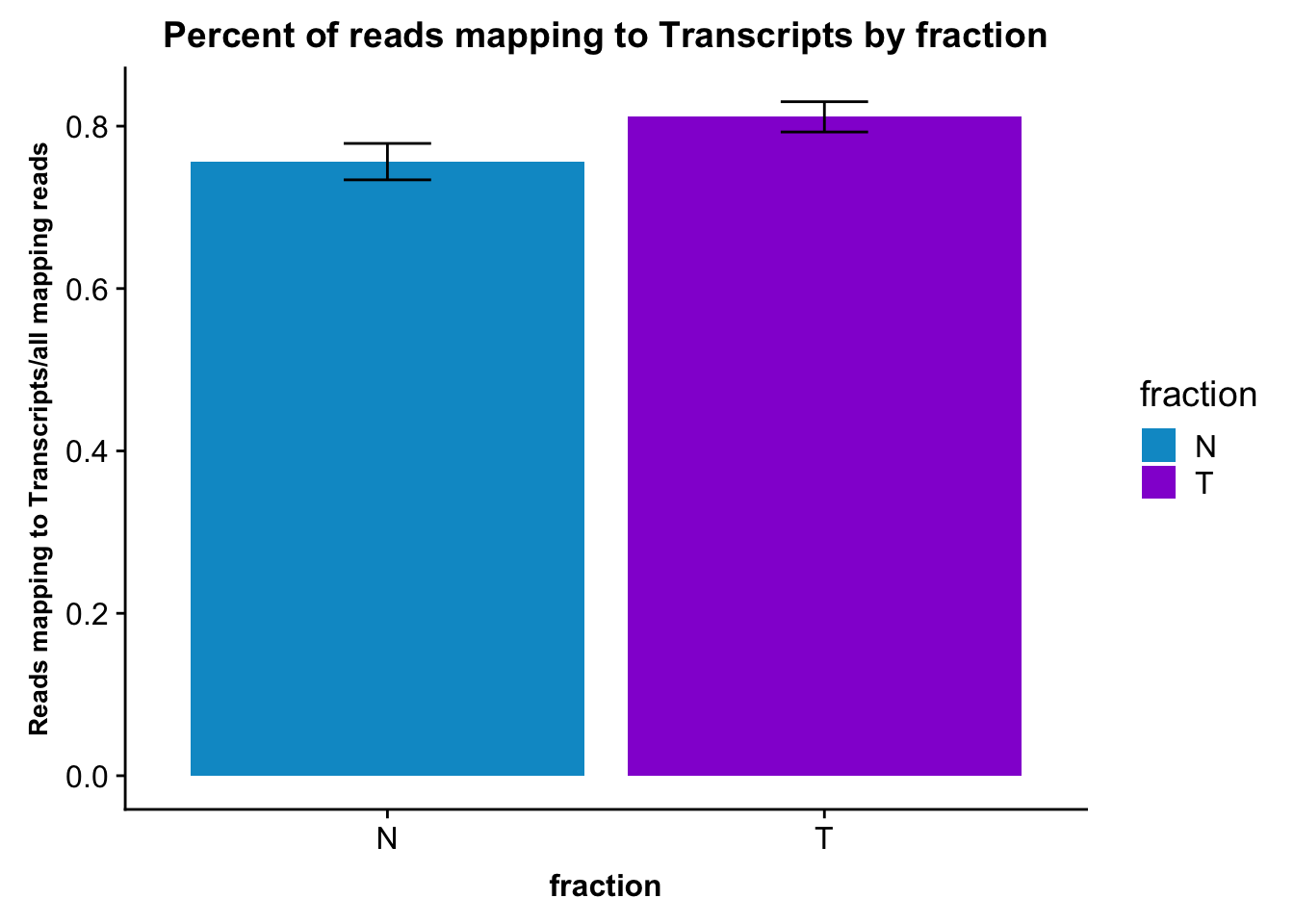
Expand here to see past versions of unnamed-chunk-60-1.png:
| Version | Author | Date |
|---|---|---|
| 6da90e9 | Briana Mittleman | 2018-12-11 |
It would be nice to have this in one plot. In order to do this I want to join the PerReadPeak from both and melt. this way the variable can be peak or transcript.
fc_peaks_sel=fc_peaks %>% select(c("line", "fraction", "PerReadPeak"))

fc_gene_peaks_sel=fc_gene_peaks %>% select(c("line", "fraction", "PerReadPeak"))

fcGene_and_Transcript=fc_peaks_sel %>% left_join(fc_gene_peaks_sel, by=c("line","fraction"))

colnames(fcGene_and_Transcript)=c("Line", "Fraction", "Peaks", "Genes")


fcGene_and_Transcript_melt=melt(fcGene_and_Transcript, id.vars=c("Line","Fraction"))


fcGene_and_Transcript_melt_sum=fcGene_and_Transcript_melt %>% group_by(Fraction,variable) %>% summarise(mean=mean(value), sd=sd(value))
reads2featuresPlot=ggplot(fcGene_and_Transcript_melt_sum,aes(x=Fraction, y=mean, fill=Fraction)) + geom_col()+ geom_errorbar(aes(ymin=mean-sd, ymax=mean+sd), width=.2)+ theme(axis.text.y = element_text(size=12),axis.title.y=element_text(size=10,face="bold"), axis.title.x=element_text(size=12,face="bold"))+ scale_fill_manual(values=c("deepskyblue3","darkviolet"))+ labs(title="Percent of reads mapping to feature by fraction", y="Reads mapping to Feature/all mapping reads") + facet_grid(~variable)
reads2featuresPlot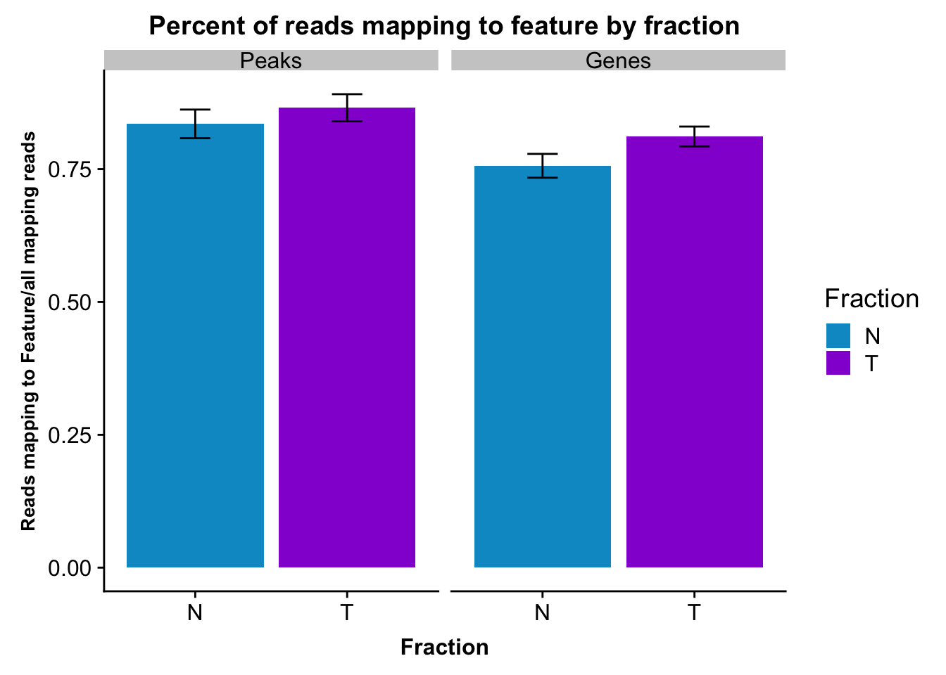
Expand here to see past versions of unnamed-chunk-62-1.png:
| Version | Author | Date |
|---|---|---|
| 6da90e9 | Briana Mittleman | 2018-12-11 |
ggsave(file="../output/plots/QC_plots/reads2featuresPlot.png", reads2featuresPlot)Saving 7 x 5 in imageMisspriming:
Sheppard et al. cited 2 other papers, Beaudoing et al 2000 and Tian et al 2005. Thet excluded reads with 6 consequitive upstream As or those with 7 in a 10nt window. They did this at the read level.
We need to think about if this is appropriate at the read level or if we can do it at the peak level
Data along transcrip bodies
I can use deeptools to plot enrichment over gene bodies. The tool will automatically scale the genes/transcripts to be the same length.
BothFracDTPlotGeneRegions.sh
#!/bin/bash

#SBATCH --job-name=BothFracDTPlotGeneRegions.sh
#SBATCH --account=pi-yangili1
#SBATCH --time=24:00:00
#SBATCH --output=BothFracDTPlotGeneRegions.out
#SBATCH --error=BothFracDTPlotGeneRegions.err
#SBATCH --partition=bigmem2
#SBATCH --mem=100G
#SBATCH --mail-type=END

module load Anaconda3
source activate three-prime-env


computeMatrix scale-regions -S /project2/gilad/briana/threeprimeseq/data/mergedBW/Total_MergedBamCoverage.bw /project2/gilad/briana/threeprimeseq/data/mergedBW/Nuclear_MergedBamCoverage.bw -R /project2/gilad/briana/genome_anotation_data/ncbiRefSeq.mRNA.named_noCHR.bed -b 1000  -a 1000 --transcript_id_designator 3 -out /project2/gilad/briana/threeprimeseq/data/UnderstandPeaksQC/BothFrac_Transcript.gz

plotHeatmap --sortRegions descend -m /project2/gilad/briana/threeprimeseq/data/UnderstandPeaksQC/BothFrac_Transcript.gz --plotTitle "Combined Reads Transcript" --heatmapHeight 7 --colorMap YlGnBu  -out /project2/gilad/briana/threeprimeseq/data/UnderstandPeaksQC/BothFrac_Transcript.png
Session information
sessionInfo()R version 3.5.1 (2018-07-02)
Platform: x86_64-apple-darwin15.6.0 (64-bit)
Running under: macOS 10.14.1
Matrix products: default
BLAS: /Library/Frameworks/R.framework/Versions/3.5/Resources/lib/libRblas.0.dylib
LAPACK: /Library/Frameworks/R.framework/Versions/3.5/Resources/lib/libRlapack.dylib
locale:
[1] en_US.UTF-8/en_US.UTF-8/en_US.UTF-8/C/en_US.UTF-8/en_US.UTF-8
attached base packages:
[1] stats graphics grDevices utils datasets methods base
other attached packages:
[1] bindrcpp_0.2.2 tximport_1.8.0 devtools_1.13.6 reshape2_1.4.3
[5] cowplot_0.9.3 workflowr_1.1.1 forcats_0.3.0 stringr_1.3.1
[9] dplyr_0.7.6 purrr_0.2.5 readr_1.1.1 tidyr_0.8.1
[13] tibble_1.4.2 ggplot2_3.0.0 tidyverse_1.2.1
loaded via a namespace (and not attached):
[1] tidyselect_0.2.4 haven_1.1.2 lattice_0.20-35
[4] colorspace_1.3-2 htmltools_0.3.6 yaml_2.2.0
[7] rlang_0.2.2 R.oo_1.22.0 pillar_1.3.0
[10] glue_1.3.0 withr_2.1.2 R.utils_2.7.0
[13] modelr_0.1.2 readxl_1.1.0 bindr_0.1.1
[16] plyr_1.8.4 munsell_0.5.0 gtable_0.2.0
[19] cellranger_1.1.0 rvest_0.3.2 R.methodsS3_1.7.1
[22] memoise_1.1.0 evaluate_0.11 labeling_0.3
[25] knitr_1.20 broom_0.5.0 Rcpp_0.12.19
[28] scales_1.0.0 backports_1.1.2 jsonlite_1.5
[31] hms_0.4.2 digest_0.6.17 stringi_1.2.4
[34] grid_3.5.1 rprojroot_1.3-2 cli_1.0.1
[37] tools_3.5.1 magrittr_1.5 lazyeval_0.2.1
[40] crayon_1.3.4 whisker_0.3-2 pkgconfig_2.0.2
[43] xml2_1.2.0 lubridate_1.7.4 assertthat_0.2.0
[46] rmarkdown_1.10 httr_1.3.1 rstudioapi_0.8
[49] R6_2.3.0 nlme_3.1-137 git2r_0.23.0
[52] compiler_3.5.1
This reproducible R Markdown analysis was created with workflowr 1.1.1